Download
1 / 18
180 likes | 313 Views
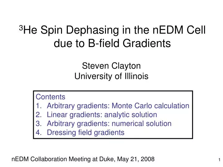
3 He Spin Dephasing in the nEDM Cell due to B-field Gradients. Steven Clayton University of Illinois. Contents Arbitrary gradients: Monte Carlo calculation Linear gradients: analytic solution Arbitrary gradients: numerical solution Dressing field gradients.

E N D
3He Spin Dephasing in the nEDM Cell due to B-field Gradients Steven Clayton University of Illinois Contents Arbitrary gradients: Monte Carlo calculation Linear gradients: analytic solution Arbitrary gradients: numerical solution Dressing field gradients nEDM Collaboration Meeting at Duke, May 21, 2008
From last collaboration meeting… H0 • long times can be simulated because collision time is much longer • requires field B(t,x,y,z) at all points in the cell y x Here, the optimized, 3D field map was (poorly) parameterized by 4th order polynomials in x, y, z. N 1000 T2 = 4202 s Long T2 can be simulated. Dressing effect can be simulated.
Diffusion Monte Carlo Simulation • Geant4 Framework • isotropic scattering from infinite-mass scattering centers. • monoenergetic. particle velocity v3 = sqrt(8 kBT/( m)) • mass m = 2.4 m3 • mean free path = 3D/v3, • D = 1.6/T7 cm2/s • Spin evolved via “quality-controlled” RK solution to Bloch equation (Numerical Recipes) • “Lambertian” reflection from walls • Scattering kernel: • cos necessary to satisfy reciprocity • results in uniform density throughout cell
N=34, l/r = 6.4 field profile With ferromagnetic shield at 300 K Known for some time that N=34 uniformity worsens in presence of ferromagnetic shield Hence, reason for design of “modified” cos θ coils with wire positions offset from nominal ASU, S. Balascuta TOSCA Caltech, M. Mendenhall nEDM November 2007 Collaboration Meeting B. Plaster
T2 due to dressing field gradients B0 y B1 x A deviation in B1 can be mapped to an equivalent deviation in B0:
Uniform Dressing Field, n34 B0 field (no FM shield) T2 from Fit 8615 386 s 1674 77 s 3896 175 s 7913 563 s 12839 815 s B1 off B1 on
Effective (Y < 1) Dashed 3He Solid UCN P. Chu (collab. meeting at ASU)
Nonuniform dressing field (B0 uniform) T2 from fit 641 +- 39 s 1.37 +- 0.2 s 871 +- 98 s 3268 +- 332 s
Redfield theory for T1, T2 Spectral density of field at spin location: ensemble average: McGregor (PRA 41, 2631) solves this for a linear gradient of H_z:
“Generalized McGregor” Diffusion equation solution in 1-D for Spectral density in terms of 3-D cosine transform over the rectangular prism cell with arbitrary B0(x,y,z): cosine transform amplitudes of Hq
Weight factors of cosine transform components For T2 • ~ 2 • 3D phase space ~ 2 For T2
Contributions to T2-1 of components of n34 B0 field (no FM shield) (nx,ny,nz) = (0,0,2)
Redfield theory calc. vs. MC simulation Redfield theory calculation: practical only for simple geometries can be applied to arbitrary (small) field non-uniformities. can be used for dressing field gradients, if B1y is mapped to B0x computationally fast for nEDM cell (using fast discrete cosine transform). ~1 CPU-second to get T1 and T2. MC: arbitrary geometries can be simulated. arbitrary fields OK. OK for arbitrary dressing fields, including Y ~ 1. ~1 CPU-hour per particle simulated to 1000 s. ~100 CPU-hours to get T1,T2.
Relaxation times for different cell lengths B0: optimized n34 coil, no FM shield. B1 off. (Redfield theory calculation)
Constraint on dressing field uniformity For a uniform gradient (à la McGregor):
Diffusive edge enhancement? Particle distributions after some elapsed time: z0 z0 • Initial positions are distributed uniformly • particle diffuses over distance Ld~sqrt(D tm) during measurement time tm. • Particles initially near a wall do not sample as much z as particles initially far from walls, if Ld is not big enough. • Smaller z smaller B longer T2 At T = 450 mK, D = 500 cm2/s. If tm = 1500 s, Ld ~ 866 cm >> Lz, but, signal decays during tm… z/Lz cell wall