Download
1 / 22
220 likes | 225 Views
Potential temperature. In situ temperature is not a conservative property in the ocean. Changes in pressure do work on a fluid parcel and changes its internal energy (or temperature) compression => warming expansion => cooling

E N D
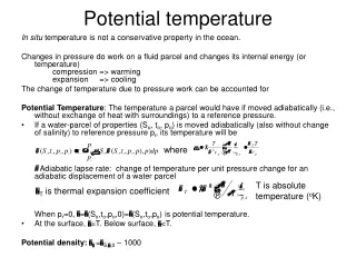
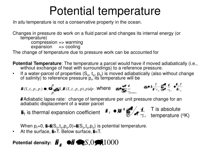
Potential temperature In situ temperature is not a conservative property in the ocean. Changes in pressure do work on a fluid parcel and changes its internal energy (or temperature) compression => warming expansion => cooling The change of temperature due to pressure work can be accounted for Potential Temperature: The temperature a parcel would have if moved adiabatically (i.e., without exchange of heat with surroundings) to a reference pressure. • If a water-parcel of properties (So, to, po) is moved adiabatically (also without change of salinity) to reference pressure pr, its temperature will be Adiabatic lapse rate: change of temperature per unit pressure change for an adiabatic displacement of a water parcel When pr=0, =(So,to,po,0)=(So,to,po) is potential temperature. • At the surface, =T. Below surface, <T. Potential density: where T is absolute temperature (oK) T is thermal expansion coefficient
A proximate formula: t in oC, S in psu, p in “dynamic km” For 30≤S≤40, -2≤T≤30, p≤ 6km, -T good to about 6% (except for some shallow values with tiny -T) In general, difference between and T is small ≈T-0.5oC for 5km
An example of vertical profiles of temperature, salinity and density
and in deep ocean Note that temperature increases in very deep ocean due to high compressibility
Definitions in-situ density anomaly: s,t,p = – 1000 kg/m3 Atmospheric-pressure density anomaly : t = s,t,0= s,t,0 – 1000 kg/m3 Specific volume anomaly: = s, t, p – 35, 0, p = s + t + s,t + s,p + t,p + s,t,p Thermosteric anomaly:s,t = s + t + s, t Potential Temperature: Potential density:=s,,0 – 1000
Static stability Simplest consideration: light on top of heavy Stable: Moving a fluid parcel (, S, T, p) from depth -z, downward adiabatically (with no heat exchange with its surroundings) and without salt exchange to depth -(z+z), its property is ( , S, T+T, p+p) and the Unstable: environment (2, S2, T2, p+p). Neutral: (This criteria is not accurate, effects of compressibility (p, T) is not counted).
Buoyant force (Archimedes’ principle): where (V, parcel’s volume) Acceleration: For the parcel: is the hydrostatic equation (where or , C is the speed of sound)
For environment: Then For small z (i.e., (z)2 and higher terms are negligible),
Static Stability: Stable: E>0 Unstable: E<0 Neutral: E=0 ( ) Therefore, in a neutral ocean, . Since E > 0 means, Note both values are negative A stable layer should have vertical density lapse rate larger then the adiabatic gradient.
A Potential Problem: E is the difference of two large numbers and hard to estimate accurately this way. g/C2 ≈ 400 x 10-8 m-1 Typical values of E in open ocean: Upper 1000 m, E~ 100 – 1000x10-8 m-1 Below 1000 m, E~ 100x10-8 m-1 Deep trench, E~ 1x10⁻⁸ m-1
Simplification of the stability expression Since For environment, For the parcel, Since and , adiabatic lapse rate, Then m-1
The effect of the pressure on the stability, which is a large number, is canceled out. (the vertical gradient of in situ density is not an efficient measure of stability). • In deep trench ∂S/∂z ~ 0, then E0 means ∂T/∂z~ - (The in situ temperature change with depth is close to adiabatic rate due to change of pressure). At 5000 m, ~ 0.14oC/1000m At 9000 m, ~ 0.19oC/1000m • At neutral condition, ∂T/∂z = - < 0. (in situ temperature increases with depth).
First approximation, , or (reliable if the calculated E > 50 x 10-8 m-1) A better approximation, (It takes into account the adiabatic change of T with pressure) When the depth is far from the surface, 4=S,,4(p=40,000kPa=4000dbar) may be used to replace .
In practice, E≈ -25 ~ -50 x 10-8 m-1 in upper 50 m. a) mixed layer is slightly unstable subtropics, increase of salinity due to evaporation, vertical overturning occurs when E ~ -16 to -64x10-8 m-1, because of the effects of heat conduction, friction, eddy diffusion, etc. b) observational errors Error of t ~ 5 x 10⁻³ The error of t at two depths t ~ 10-2 for z=z1-z2=20 m.
Cold water is more compressible than warm water (Fig.2.1c) Because of the existence of salinity, two water parcels at the same pressure can have the same density but differ in temperature and hence in compressibility When such two parcels are moved together to another pressure, they will have different densities in their new locations is the density of a parcel lifted to sea surface. If two parcels with close densities but different temperatures are lifted from deep depth, their relative density changes may change their “apparent” stability. It is more accurate to use reference level closer to (within 500m) the in situ position (e.g., 4 for deep ocean)
Buoyancy frequency (Brunt-Väisälä frequency, N) We have known that ,(depending on z, restoring force) Since z is the vertical displacement of the parcel, then or Its solution has the form where (radians/s)2 N is the maximum frequency of internal waves in water of stability E. Period: E=1000 x 10-8 m-1, =10 min E=100 x 10-8 m-1, =33 min E=1 x 10⁻⁸ m-1, ≈6hr