Download
1 / 57
570 likes | 729 Views
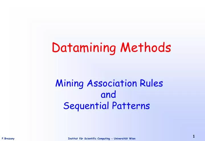
Datamining Methods Mining Association Rules and Sequential Patterns. KDD (Knowledge Discovery in Databases) Process. Data Mining. Clean, Collect, Summarize. Data Preparation. Training Data. Data Warehouse. Model, Patterns. Verification & Evaluation. Operational

E N D
Datamining Methods Mining Association Rules and Sequential Patterns
KDD (Knowledge Discovery in Databases) Process Data Mining Clean, Collect, Summarize Data Preparation Training Data Data Warehouse Model, Patterns Verification & Evaluation Operational Databases
Association rule mining finds interesting association orcorrelation relationships among a large set of data items. This can help in many business decision making processes: store layout, catalog design, and customer segmentation based on buying paterns. Another important field: medical applications. Market basket analysis - a typical example of association rule mining. How can we find association rules from large amounts of data? Which association rules are the most interesting. How can we help or guide the mining procedures? Mining Association Rules
Given a set of database transactions, where each transaction is a set of items, an association rule is an expressionX Ywhere X and Y are sets of items (literals). The intuitive meaningof the rule: transactions in the database which contain the items in X tend to also contain the items in Y. Example: 98% of customers who purchase tires and auto accessories also buy some automotive services; here 98% is called the confidence of the rule. The support of the ruleis the percentage of transactions that contain both X and Y. The problem of mining association rules is to find all rules that satisfy a user-specified minimum support and minimum confidence. Informal Introduction
Basic Concepts Let J = (i1, i2, ..., im) be a set of items.Typically, the items are identifiers of individuals articles (pro- ducts (e.g., bar codes). Let D, the task relevant data, be a set of database transactions where each transaction T is a set of items such that T J. Let A be a set of items: a transaction T is said to contain A if and only if A T, An association rule is an implication of the form A B, where A J, B J, and A B = . The rule A B holds in the transaction set D with supports, where s is the percentage of transactions in D that contain A B (i.e. both A and B). This is the probability, P(A B).
Basic Concepts (Cont.) The rule A B has confidencec in the transaction set D if c is the percentage of transactions in D containing A that also contain B - the conditional probability P(B|A). Rules that satisfy both a minimum support threshold (min_sup) and a minimum confidence threshold (min_conf) are called strong. A set of items is referred to as an itemset. An itemset that contains k items is a k-itemset. The occurence frequency of an itemset is the number of transactions that contain the itemset.
Basic Concepts - Example transaction purchased items 1 bread, coffee, milk, cake 2 coffee, milk, cake 3 bread, butter, coffee, milk 4 milk, cake 5 bread, cake 6 bread X = {coffee, milk} R = {coffee, cake, milk} support of X = 3 from 6 = 50% support of R = 2 from 6 = 33% Support of “milk, coffee” “cake” equals to support of R = 33% Confidence of “milk, coffee” “cake” = 2 from 3 = 67% [=support(R)/support(X)]
Basic Concepts (Cont.) An itemset satisfies minimum support if the occurrence fre- quency of the itemset is greater than or equal to the product of min_sup and the total number of transactions in D. The number of transactions required for the itemset to satis- fy minimum support is therefore referred to as the minimum support count. If an itemset satisfy minimum support, then it is a frequent itemset. The set of frequent k-itemsets is commonly denoted by Lk. Association rule mining is a two-step process: 1. Find all frequent itemsets. 2. Generate strong association rules from the frequent itemsets.
Based on the types of values handled in the rule:If a rule concerns associations between the presence or absence of items, it is a Boolean association rule. For example:computer financial_management_software [support = 2%, confidence = 60%]If a rule describes associations between quantitative items or attributes, then it is a quantitative associa-tion rule. For example:age(X, “30..39”) and income(X,”42K..48K”) buys(X, high resolution TV)Note that the quantitative attributes, age and income,have been discretized. Association Rule Classification
Based on the dimensions of data involved in the rule:If the items or attributes in an association rule refe-rence only one dimension, then it is a single dimensional association rule. For example:buys(X,”computer”) buys (X, “financial manage- ment software”)The above rule refers to only one dimension, buys.If a rule references two or more dimensions, such as buys, time_of_transaction, and customer_category, then it is a multidimensional association rule.The second rule on the previous slide is a 3-dimensional ass. rule since it involves 3 dimensions: age, income, and buys. Association Rule Classification (Cont.)
Based on the levels of abstractions involved in the rule set:Suppose that a set of association rules minded includes:age(X,”30..39”) buys(X, “laptop computer”) age(X,”30..39”) buys(X, “computer”) In the above rules, the items bought are referenced at different levels of abstraction. (E.g., “computer” is a higher-level abstraction of “laptop computer” .) Such ru-les are called multilevel association rules.Single-level association rules refer one abstraction level only. Association Rule Classification (Cont.)
Mining Single-Dimensional Boolean Association Rules from Transactional Databases This is the simplest form of association rules (used in market basket analysis. We present Apriori, a basic algorithm for finding frequent itemsets. Its name – it uses prior knowledge of frequent itemset properties (explained later). Apriori employs a iterative approach known as a level-wise search, where k-itemsets are used to explore (k + 1)-itemsets. First, the set of frequent 1-items, L1, is found. L1 is used to find L2, the set of frequent 2-itemsets, which is used to find L3, and so on, until no more frequent k-itemsets can be found. The finding of each Lk requires one full scan of the database. The Apriori property is used to reduce the search space.
The Apriori Property All nonempty subsets of a frequent itemset must also be frequent. If an itemset I does not satisfy the minimum support threshold, min_sup, then I is not frequent, that is, P(I) < min_sup. If an item A is added to the itemset I, then the resulting itemset (i.e., I A ) cannot occur more frequently than I. Therefore, I A is not frequent either, that is, P (I A ) < min_sup. How is the Apriori property used in the algorithm? To understand this, let us look at how Lk-1 is used to find Lk.A two-step process is followed, consisting of join and prune actions. These steps are explained on the next slides,
The Apriori Algorithm – the Join Step To find Lk, a set of candidate k-itemsets is generated by joining Lk-1 with itself. This set of candidates is denoted by Ck. Let l1and l2 be itemsets in Lk-1. The notation li[j] refers to the jth item in li (e.g., li[k-2] refers to the second to the last item in l1). Apriori assumes that items within a transaction or itemset are sorted in lexicographic order. The join Lk-1joinLk-1, is performed, where members of Lk-1 are joinable if their first (k-2) items are in common. That is, members l1 and l2 of Lk-1 are joined if (l1[1] = l2[1] ) (l1[2] = l2[2] ) ... (l1[k-2] = l2[k-2] ) (l1[k-1]<l2[k-1] ) . The condition (l1[k-1]<l2[k-1] ) simply ensures that no duplicates are generated. The resulting itemset: l1[1]l1[2] ) ... l1[k-1]l2[k-1] .
The Apriori Algorithm – the Join Step (2) Illustration by an example p Lk-1 = ( 1 2 3) || || Join: Result Ck = ( 1 2 3 4) || || q Lk-1 = ( 1 2 4) Each frequent k-itemset p is always extended by the last item of all frequent itemsets q which have the same first k-1 items as p .
The Apriori Algorithm – the Prune Step Ck is a superset of Lk, that is, its members may or may not be frequent, but all of the frequent k-items are included in Ck. A scan of the database to determine the count of each candidate in Ck would result in the determination of Lk. Ck can be huge, and so this could involve heavy computation. To reduce the size of Ck, the Apriori property is used as follows. Any (k-1)-itemset that is not frequent cannot be a subset of a frequent k-itemset. Hence, if any (k-1)-subset of a candidate k-itemset is not in Lk-1, then the candidate cannot be frequent either and so can be removed from Ck. The above subset testing can be done quickly by maintaining a hash tree of all frequent itemsets.
The Apriori Algorithm - Example Let’s look at a concrete example of Apriori, based on the AllElectronics transaction database D, shown below. There are nine transactions in this database, e.i., |D| = 9. We use the next figure to illus- trate the fin- ding of fre- quent itemsets in D. TID List of item_Ids T100 I1, I2, I5 T200 I2, I4 T300 I2, I3 T400 I1, I2, I4 T500 I1, I3 T600 I2, I3 T700 I1, I3 T800 I1, I2, I3, I5 T900 I1, I2, I3
Generation of CKand LK(min.supp. count=2) Scan D for count of each candidate- scan Itemset Sup. count {I1} 6 {I2} 7 {I3} 6 {I4} 2 {I5} 2 Itemset Sup. count {I1} 6 {I2} 7 {I3} 6 {I4} 2 {I5} 2 Compare candidate support count with minimum support count - compare C1 L1 Itemset {I1,I2} {I1,I3} {I1,I4} {I1,I5} {I2,I3} {I2,I4} {I2,I5} {I3,I4} {I3,I5} {I4,I5} Itemset Sup. count {I1,I2} 4 {I1,I3} 4 {I1,I4} 1 {I1,I5} 2 {I2,I3} 4 {I2,I4} 2 {I2,I5} 2 {I3,I4} 0 {I3,I5} 1 {I4,I5} 0 Itemset Sup. count {I1,I2} 4 {I1,I3} 4 {I1,I5} 2 {I2,I3} 4 {I2,I4} 2 {I2, I5} 2 Generate C2 candidates from L1 Scan Compare L2 C2 C2
Generation of CKand LK(min.supp. count=2) Generate C3 candidates from L2 Itemset {I1,I2,I3} {I1,I2,I5} Itemset Sup. Count {I1,I2,I3} 2 {I1,I2,I5} 2 Itemset Sup. Count {I1,I2,I3} 2 {I1,I2,I5} 2 Scan Compare C3 C3 L3
In the 1st iteration, each item is a member of C1. The algorithm simply scan all the transactions in order to count the number of occurrences of each item. Suppose that the minimum transaction support count (min_sup = 2/9 = 22%). L1 can then be determined. C2 =L1joinL1. The transactions in D are scanned and the support count of each candidate itemset in C2, as shown in the middle table of the second row in the last figure. The set of frequent 2-itemsets, L2, is then determined, consisting of those candidate 2-itemsets in C2 having minimum support. Algorithm Application Description
The generation of C3 =L2joinL2 is detailed in the next figure. Based on the Apriori property that all subsets of a frequent itemset must also be frequent, we can determine that the four latter candidates cannot possibly be frequent. We therefore remove them from C3. The transactions in D are scanned in order to determine L3 , consisting of those candidate 3-itemsets in C3 having minimum support. C4 =L3joinL3 , after the pruning C4 = Ø. Algorithm Application Description (2)
Example: Generation C3 from L2 1. Join: C3=L2L2 = {{I1,I2},{I1,I3},{I1,I5}, {I2,I3},{I2,I4}, {I2,I5}} {I1,I2}, {I1,I3}, {I1,I5}, {I2,I3},{I2,I4}, {I2,I5}} = {{I1,I2,I3}, {I1,I2,I5}, {I1,I3,I5}, {I2,I3,I4}, {I2,I3,I5}, {I2,I4,I5}}. 2. Prune using the Apriori property: All nonempty subsets of a frequent itemset must also be frequent. The 2-item subsets of {I1,I2,I3} are {I1,I2}, {I1,I3}, {I2,I3}, and they all are members of L2. Therefore, keep {I1,I2,I3} in C3. The 2-item subsets of {I1,I2,I5} are {I1,I2}, {I1,I5}, {I2,I5}, and they all are members of L2. Therefore, keep {I1,I2,I5} in C3. Using the same analysis remove other 3-items from C3. 3. Therefore, C3 = {{I1,I2,I3}, {I1,I2,I5}} after pruning.
Generating Association Rules from Frequent Items We generate strong association rules - they satisfy both minimum support and minimum confidence. support_count(A B) confidence ( A B ) = P(B|A) = ------------------------- support_count(A) where support_count(A B) is the number of transactions containing the itemsets A B, and support_count(A) is the number of transactions containing the itemset A.
Generating Association Rules from Frequent Items (Cont.) Based on the equations on the previous slide, association rules can be generated as follows: - For each frequent itemset l , generate all nonempty subsets of l. - For every nonempty subset s of l, output the rule “s (l - s)” support_count(l) if ----------------- min_conf, where min_conf is minimum support_count(s) confidence threshold.
Generating Association Rules - Example Suppose that the transactional data for AllElectronics contain the frequent itemset l = {I1,I2,I5}. The resulting rules are: I1 I2 I5, confidence = 2/4 = 50% I1 I5 I2, confidence = 2/2 = 100% I2 I5 I1, confidence = 2/2 = 100% I1 I2 I5, confidence = 2/6 = 33% I2 I1 I5, confidence = 2/7 = 29% I5 I1 I2, confidence = 2/2 = 100% If the minimum confidence threshold is, say, 70%, then only the second, third, and the last rules above are output, since these are the only ones generated that are strong.
Multilevel (Generalized) Association Rules For many applications, it is difficult to find strong associations among data items at low or primitive levels of abstraction due to sparsity of data in multidimensional space. Strong associations discovered at high concept levels may represent common sense knowledge. However, what may represent common sense to one user may seem novel to another. Therefore, data mining systems should provide capabilities to mine association rules at multiple levels of abstraction and traverse easily among different abstraction spaces.
Multilevel (Generalized) Association Rules - Example Suppose we are given the following task-relevant set of transactional data for sales at the computer department of an AllElectronics branch, showing the items purchased for each transaction TID. TID Items purchased T1 IBM desktop computer, Sony b/w printer T2 Microsoft educational software, Microsoft financial software T3 Logitech mouse computer accessory, Ergoway wrist pad accessory T4 IBM desktop computer, Microsoft financial software T5 IBM desktop computer . . . . . . Table Transactions
A Concept Hierarchy for our Example Level 0 all Computer accessory computer software printer wrist pad mouse desktop laptop educational financial color b/w ... ... ... ... ... ... ... HP Sony Ergoway Logitech IBM Microsoft ... ... ... Level 3
Example (Cont.) The items in Table Transactions are at the lowest level of the concept hierarchy. It is difficult to find interesting purchase patterns at such raw or primitive level data. If, e.g., “IBM desktop computer” or “Sony b/w printer” each occurs in a very small fraction of the transactions, then it may be difficult to find strong associations involving such items. In other words, it is unlikely that the itemset “{IBM desktop computer, Sony b/w printer}” will satisfy minimum support. Itemsets containing generalized items, such as “{IBM desktop computer, b/w printer}” and “{computer, printer}” are more likely to have minimum support. Rules generated from association rule mining with concept hie- rarchies are called multiple-level or multilevel or generalized association rules.
Need: Huge Transaction Datasets (10s of TB) Large Number of Candidates. Data Distribution: Partition the Transaction Database, or Partition the Candidates, or Both Parallel Formulation of Association Rules
Each Processor has complete candidate hash tree. Each Processor updates its hash tree with local data. Each Processor participates in global reduction to get global counts of candidates in the hash tree. Multiple database scans per iteration are required if hash tree too big for memory. Parallel Association Rules: Count Distribution (CD)
{1,2} 7 {1,2} 0 {1,2} 2 {1,3} 3 {1,3} 2 {1,3} 5 {2,3} 1 {2,3} 8 {2,3} 3 {3,4} 1 {3,4} 2 {3,4} 7 {5,8} 2 {5,8} 9 {5,8} 6 CD: Illustration P0 P1 P2 N/p N/p N/p Global Reduction of Counts
Candidate set is partitioned among the processors. Once local data has been partitioned, it is broadcast to all other processors. High Communication Cost due to data movement. Redundant work due to multiple traversals of the hash trees. Parallel Association Rules: Data Distribution (DD)
N/p N/p N/p Count Count Count {5,8} 17 DD: Illustration Data Broadcast P0 P1 P2 Remote Data Remote Data Remote Data {1,2} 9 12 {2,3} {1,3} 10 {3,4} 10 All-to-All Broadcast of Candidates
Markup language (XML) to describe data mining models PMML describes: the inputs to data mining models the transformations used prior to prepare data for data mining The parameters which define the models themselves Predictive Model Markup Language - PMML
Model attributes (1) <xs:element name="AssociationModel"> <xs:complexType> <xs:sequence> <xs:element minOccurs="0" maxOccurs="unbounded" ref="Extension" /> <xs:element ref="MiningSchema" /> <xs:element minOccurs="0" maxOccurs="unbounded" ref="Item" /> <xs:element minOccurs="0" maxOccurs="unbounded" ref="Itemset" /> <xs:element minOccurs="0" maxOccurs="unbounded" ref="AssociationRule" /> <xs:element minOccurs="0" maxOccurs="unbounded" ref="Extension" /> </xs:sequence> … PMML 2.1 – Association Rules (1)
1. Model attributes (2) <xs:attribute name="modelName" type="xs:string" /> <xs:attribute name="functionName" type="MINING-FUNCTION“ use="required"/> <xs:attribute name="algorithmName" type="xs:string" /> <xs:attribute name="numberOfTransactions" type="INT-NUMBER" use="required" /> <xs:attribute name="maxNumberOfItemsPerTA" type="INT-NUMBER" /> <xs:attribute name="avgNumberOfItemsPerTA" type="REAL-NUMBER" /> <xs:attribute name="minimumSupport" type="PROB-NUMBER" use="required" /> <xs:attribute name="minimumConfidence" type="PROB-NUMBER" use="required" /> <xs:attribute name="lengthLimit" type="INT-NUMBER" /> <xs:attribute name="numberOfItems" type="INT-NUMBER" use="required" /> <xs:attribute name="numberOfItemsets" type="INT-NUMBER" use="required" /> <xs:attribute name="numberOfRules" type="INT-NUMBER" use="required" /> </xs:complexType> </xs:element> PMML 2.1 – Association Rules (2)
2. Items <xs:element name="Item"> <xs:complexType> <xs:attribute name="id" type="xs:string" use="required" /> <xs:attribute name="value" type="xs:string" use="required" /> <xs:attribute name="mappedValue" type="xs:string" /> <xs:attribute name="weight" type="REAL-NUMBER" /> </xs:complexType> </xs:element> PMML 2.1 – Association Rules (3)
3. ItemSets <xs:element name="Itemset"> <xs:complexType> <xs:sequence> <xs:element minOccurs="0" maxOccurs="unbounded" ref="ItemRef“ /> <xs:element minOccurs="0" maxOccurs="unbounded" ref="Extension“ /> </xs:sequence> <xs:attribute name="id" type="xs:string" use="required" /> <xs:attribute name="support" type="PROB-NUMBER" /> <xs:attribute name="numberOfItems" type="INT-NUMBER" /> </xs:complexType> </xs:element> PMML 2.1 – Association Rules (4)
4. AssociationRules <xs:element name="AssociationRule"> <xs:complexType> <xs:sequence> <xs:element minOccurs="0" maxOccurs="unbounded" ref="Extension" /> </xs:sequence> <xs:attribute name="support" type="PROB-NUMBER" use="required" /> <xs:attribute name="confidence" type="PROB-NUMBER" use="required" /> <xs:attribute name="antecedent" type="xs:string" use="required" /> <xs:attribute name="consequent" type="xs:string" use="required" /> </xs:complexType> </xs:element> PMML 2.1 – Association Rules (5)
<?xml version="1.0" ?> <PMML version="2.1" > <DataDictionary numberOfFields="2" > <DataField name="transaction" optype="categorical" /> <DataField name="item" optype="categorical" /> </DataDictionary> <AssociationModel functionName="associationRules" numberOfTransactions="4" numberOfItems=“4" minimumSupport="0.6" minimumConfidence="0.3" numberOfItemsets=“7" numberOfRules=“3"> <MiningSchema> <MiningField name="transaction"/> <MiningField name="item"/> </MiningSchema> PMML example model for AssociationRules (1)
<!-- four items - input data --> <Item id="1" value=“PC" /> <Item id="2" value=“Monitor" /> <Item id="3" value=“Printer" /> <Item id=“4" value=“Notebook" /> <!-- three frequent 1-itemsets --> <Itemset id="1" support="1.0" numberOfItems="1"> <ItemRef itemRef="1" /> </Itemset> <Itemset id="2" support="1.0" numberOfItems="1"> <ItemRef itemRef=“2" /> </Itemset> <Itemset id=“3" support="1.0" numberOfItems="1"> <ItemRef itemRef="3" /> </Itemset> PMML example model for AssociationRules (2)
<!-- three frequent 2-itemset --> <Itemset id=“4" support="1.0" numberOfItems="2"> <ItemRef itemRef="1" /> <ItemRef itemRef=“2" /> </Itemset> <Itemset id=“5" support="1.0" numberOfItems="2"> <ItemRef itemRef="1" /> <ItemRef itemRef=“3" /> </Itemset> <Itemset id=“6" support="1.0" numberOfItems="2"> <ItemRef itemRef=“2" /> <ItemRef itemRef="3" /> </Itemset> PMML example model for AssociationRules (3)
<!-- one frequent 3-itemset --> <Itemset id=“7" support="0.9" numberOfItems=“3"> <ItemRef itemRef="1" /> <ItemRef itemRef=“2" /> <ItemRef itemRef="3" /> </Itemset> <!-- three rules satisfy the requirements – the output --> <AssociationRule support="0.9“ confidence="0.85“ antecedent=“4" consequent=“3" /> <AssociationRule support="0.9" confidence="0.75" antecedent=“1" consequent=“6" /> <AssociationRule support="0.9" confidence="0.70" antecedent=“6" consequent="1" /> </AssociationModel> </PMML> PMML example model for AssociationRules (4)
Visualization of Association Rules (1) 1. Table Format
2. Directed Graph Visualization of Association Rules (2) PC Printer Monitor Monitor PC Printer Printer PC Monitor
Visualization of Association Rules (3) 3. 3-D Visualisation
Discovering sequential patterns is a relatively new data mining problem. The input data is a set of sequences, called data-sequences. Each data-sequence is a list of transactions where each transaction is a set of items. Typically, there is a transaction time associated with each transaction. A sequential pattern also consists of a list of sets of items. The problem is to find all sequential patterns with a user-specified minimum support , where the support of a sequential pattern is a percentage of data-sequences that contain the pattern. Mining Sequential Patterns