Mining Association Rules

Mining Association Rules Part II

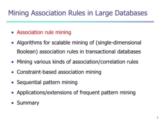
Data Mining Overview • Data Mining • Data warehouses and OLAP (On Line Analytical Processing.) • Association Rules Mining • Clustering: Hierarchical and Partitional approaches • Classification: Decision Trees and Bayesian classifiers • Sequential Patterns Mining • Advanced topics: outlier detection, web mining

Problem Statement • I = {i1, i2, …, im}: a set of literals, called items • Transaction T: a set of items s.t. TI • Database D: a set of transactions • A transaction contains X, a set of items in I, if X T • An association rule is an implication of the form X  Y, where X,Y I • The rule X  Y holds in the transaction set D with confidence c if c% of transactions in D that contain X also contain Y • The rule X  Y has support s in the transaction set D if s% of transactions in D contain X Y • Find all rules that have support and confidence greater than user-specified min support and min confidence

Problem Decomposition 1. Find all sets of items that have minimum support (frequent itemsets) 2. Use the frequent itemsets to generate the desired rules

Mining Frequent Itemsets: the Key Step • Find the frequent itemsets: the sets of items that have minimum support • A subset of a frequent itemset must also be a frequent itemset • i.e., if {AB} isa frequent itemset, both {A} and {B} should be a frequent itemset • Iteratively find frequent itemsets with cardinality from 1 to k (k-itemset) • Use the frequent itemsets to generate association rules.

The Apriori Algorithm • Lk: Set of frequent itemsets of size k (those with min support) • Ck: Set of candidate itemset of size k (potentially frequent itemsets) L1 = {frequent items}; for(k = 1; Lk !=; k++) do begin Ck+1 = candidates generated from Lk; for each transaction t in database do increment the count of all candidates in Ck+1 that are contained in t Lk+1 = candidates in Ck+1 with min_support end returnkLk;

How to Generate Candidates? • Suppose the items in Lk-1 are listed in order • Step 1: self-joining Lk-1 insert intoCk select p.item1, p.item2, …, p.itemk-1, q.itemk-1 from Lk-1 p, Lk-1 q where p.item1=q.item1, …, p.itemk-2=q.itemk-2, p.itemk-1 < q.itemk-1 • Step 2: pruning forall itemsets c in Ckdo forall (k-1)-subsets s of c do if (s is not in Lk-1) then delete c from Ck

How to Count Supports of Candidates? • Why counting supports of candidates a problem? • The total number of candidates can be very huge • One transaction may contain many candidates • Method: • Candidate itemsets are stored in a hash-tree • Leaf node of hash-tree contains a list of itemsets and counts • Interior node contains a hash table • Subset function: finds all the candidates contained in a transaction

Hash-tree:search • Given a transaction T and a set Ck find all of its members contained in T • Assume an ordering on the items • Start from the root, use every item in T to go to the next node • If you are at an interior node and you just used item i, then use each item that comes after i in T • If you are at a leaf node check the itemsets

Is Apriori Fast Enough? — Performance Bottlenecks • The core of the Apriori algorithm: • Use frequent (k – 1)-itemsets to generate candidate frequent k-itemsets • Use database scan and pattern matching to collect counts for the candidate itemsets • The bottleneck of Apriori: candidate generation • Huge candidate sets: • 104 frequent 1-itemset will generate 107 candidate 2-itemsets • To discover a frequent pattern of size 100, e.g., {a1, a2, …, a100}, one needs to generate 2100  1030 candidates. • Multiple scans of database: • Needs (n +1 ) scans, n is the length of the longest pattern

Max-Miner • Max-miner finds long patterns efficiently: the maximal frequent patterns • Instead of checking all subsets of a long pattern try to detect long patterns early • Scales linearly to the size of the patterns

Max-Miner: the idea Set enumeration tree of an ordered set f 1 3 4 2 Pruning: (1) set infrequency (2) Superset frequency 1,2 1,3 1,4 2,3 2,4 3,4 1,2,3 2,3,4 1,2,4 1,3,4 Each node is a candidate group g h(g) is the head: the itemset of the node t(g) tail: an ordered set that contains all items that can appear in the subnodes 1,2,3,4 Example: h({1}) = {1} and t({1}) = {2,3,4}

Max-miner pruning • When we count the support of a candidate group g, we compute also the support for h(g), h(g) t(g) and h(g) {i} for each i in t(g) • If h(g) t(g) is frequent, then stop expanding the node g and report the union as frequent itemset • If h(g) {i} is infrequent, then remove i from all subnodes (just remove i from any tail of a group after g) • Expand the node g by one and do the same

The algorithm Max-Miner Set candidate groups C {} Set of Itemsets F {Gen-Initial-Groups(T,C)} while C not empty do scan T to count the support of all candidate groups in C for each g in C s.t. h(g) U t(g) is frequent do F  F U {h(g) U t(g)} Set candidate groups Cnew{ } for each g in C such that h(g) U t(g) is infrequent do F F U {Gen-sub-nodes(g, Cnew)} C  Cnew remove from F any itemset with a proper superset in F remove from C any group g s.t. h(g) U t(g) has a superset in F return F

The algorithm (2) Gen-Initial-Groups(T, C) scan T to obtain F1, the set of frequent 1-itemsets impose an ordering on items in F1 for each item i in F1 other than the greatest itemset do let g be a new candidate with h(g) = {i} and t(g) = {j | j follows i in the ordering} C C U {g} return the itemset F1 (an the C of course) Gen-sub-nodes(g, C) /* generation of new itemsets at the next level*/ remove any item i from t(g) if h(g) U {i} is infrequent reorder the items in t(g) for each i in t(g) other than the greatest do let g’ be a new candidate with h(g’) = h(g) U {i} and t(g’) = {j | j in t(g) and j is after i in t(g)} C  C U {g’} return h(g) U {m} where m is the greatest item in t(g) or h(g) if t(g) is empty

Item Ordering • By re-ordering items we try to increase the effectiveness of frequency-pruning • Very frequent items have higher probability to be contained in long patterns • Put these item at the end of the ordering, so they appear in many tails

Mining Frequent Patterns Without Candidate Generation • Compress a large database into a compact, Frequent-Pattern tree (FP-tree) structure • highly condensed, but complete for frequent pattern mining • avoid costly database scans • Develop an efficient, FP-tree-based frequent pattern mining method • A divide-and-conquer methodology: decompose mining tasks into smaller ones • Avoid candidate generation: sub-database test only!

{} Header Table Item frequency head f 4 c 4 a 3 b 3 m 3 p 3 f:4 c:1 c:3 b:1 b:1 a:3 p:1 m:2 b:1 p:2 m:1 Construct FP-tree from a Transaction DB TID Items bought (ordered) frequent items 100 {f, a, c, d, g, i, m, p}{f, c, a, m, p} 200 {a, b, c, f, l, m, o}{f, c, a, b, m} 300 {b, f, h, j, o}{f, b} 400 {b, c, k, s, p}{c, b, p} 500{a, f, c, e, l, p, m, n}{f, c, a, m, p} min_support = 0.5 • Steps: • Scan DB once, find frequent 1-itemset (single item pattern) • Order frequent items in frequency descending order • Scan DB again, construct FP-tree

Benefits of the FP-tree Structure • Completeness: • never breaks a long pattern of any transaction • preserves complete information for frequent pattern mining • Compactness • reduce irrelevant information—infrequent items are gone • frequency descending ordering: more frequent items are more likely to be shared • never be larger than the original database (if not count node-links and counts) • Example: For Connect-4 DB, compression ratio could be over 100

Mining Frequent Patterns Using FP-tree • General idea (divide-and-conquer) • Recursively grow frequent pattern path using the FP-tree • Method • For each item, construct its conditional pattern-base, and then its conditional FP-tree • Repeat the process on each newly created conditional FP-tree • Until the resulting FP-tree is empty, or it contains only one path(single path will generate all the combinations of its sub-paths, each of which is a frequent pattern)

Major Steps to Mine FP-tree • Construct conditional pattern base for each node in the FP-tree • Construct conditional FP-tree from each conditional pattern-base • Recursively mine conditional FP-trees and grow frequent patterns obtained so far • If the conditional FP-tree contains a single path, simply enumerate all the patterns

Header Table Item frequency head f 4 c 4 a 3 b 3 m 3 p 3 {} f:4 c:1 c:3 b:1 b:1 a:3 p:1 m:2 b:1 p:2 m:1 Step 1: From FP-tree to Conditional Pattern Base • Starting at the frequent header table in the FP-tree • Traverse the FP-tree by following the link of each frequent item • Accumulate all of transformed prefix paths of that item to form a conditional pattern base Conditional pattern bases item cond. pattern base c f:3 a fc:3 b fca:1, f:1, c:1 m fca:2, fcab:1 p fcam:2, cb:1

Properties of FP-tree for Conditional Pattern Base Construction • Node-link property • For any frequent item ai,all the possible frequent patterns that contain ai can be obtained by following ai's node-links, starting from ai's head in the FP-tree header • Prefix path property • To calculate the frequent patterns for a node ai in a path P, only the prefix sub-path of ai in P need to be accumulated, and its frequency count should carry the same count as node ai.

{} f:3 c:3 a:3 m-conditional FP-tree Step 2: Construct Conditional FP-tree • For each pattern-base • Accumulate the count for each item in the base • Construct the FP-tree for the frequent items of the pattern base {} • m-conditional pattern base: • fca:2, fcab:1 Header Table Item frequency head f 4 c 4 a 3 b 3 m 3 p 3 f:4 c:1 All frequent patterns concerning m m, fm, cm, am, fcm, fam, cam, fcam c:3 b:1 b:1   a:3 p:1 m:2 b:1 p:2 m:1

Item Conditional pattern-base Conditional FP-tree p {(fcam:2), (cb:1)} {(c:3)}|p m {(fca:2), (fcab:1)} {(f:3, c:3, a:3)}|m b {(fca:1), (f:1), (c:1)} Empty a {(fc:3)} {(f:3, c:3)}|a c {(f:3)} {(f:3)}|c f Empty Empty Mining Frequent Patterns by Creating Conditional Pattern-Bases

{} f:3 c:3 am-conditional FP-tree {} f:3 c:3 a:3 m-conditional FP-tree Step 3: Recursively mine the conditional FP-tree Cond. pattern base of “am”: (fc:3) {} Cond. pattern base of “cm”: (f:3) f:3 cm-conditional FP-tree {} Cond. pattern base of “cam”: (f:3) f:3 cam-conditional FP-tree

Single FP-tree Path Generation • Suppose an FP-tree T has a single path P • The complete set of frequent pattern of T can be generated by enumeration of all the combinations of the sub-paths of P {} All frequent patterns concerning m m, fm, cm, am, fcm, fam, cam, fcam f:3  c:3 a:3 m-conditional FP-tree

Principles of Frequent Pattern Growth • Pattern growth property • Let  be a frequent itemset in DB, B be 's conditional pattern base, and  be an itemset in B. Then    is a frequent itemset in DB iff  is frequent in B. • “abcdef ” is a frequent pattern, if and only if • “abcde ” is a frequent pattern, and • “f ” is frequent in the set of transactions containing “abcde ”

Why Is Frequent Pattern Growth Fast? • Our performance study shows • FP-growth is an order of magnitude faster than Apriori, and is also faster than tree-projection • Reasoning • No candidate generation, no candidate test • Use compact data structure • Eliminate repeated database scan • Basic operation is counting and FP-tree building

FP-growth vs. Apriori: Scalability With the Support Threshold Data set T25I20D10K

FP-growth vs. Tree-Projection: Scalability with Support Threshold Data set T25I20D100K

Presentation of Association Rules (Table Form )

Visualization of Association Rule Using Plane Graph

Visualization of Association Rule Using Rule Graph

Iceberg Queries • Icerberg query: Compute aggregates over one or a set of attributes only for those whose aggregate values is above certain threshold • Example: selectP.custID, P.itemID, sum(P.qty) from purchase P group by P.custID, P.itemID havingsum(P.qty) >= 10 • Compute iceberg queries efficiently by Apriori: • First compute lower dimensions • Then compute higher dimensions only when all the lower ones are above the threshold

Mining Association Rules