Assumption of normality

1. Assumption of normality Assumption of normality Transformations Assumption of normality script Practice problems

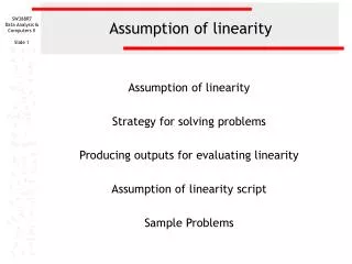
2. Assumption of Normality • Many of the statistical methods that we will apply require the assumption that a variable or variables are normally distributed. • With multivariate statistics, the assumption is that the combination of variables follows a multivariate normal distribution. • Since there is not a direct test for multivariate normality, we generally test each variable individually and assume that they are multivariate normal if they are individually normal, though this is not necessarily the case.

3. Assumption of Normality:Evaluating Normality There are both graphical and statistical methods for evaluating normality. • Graphical methods include the histogram and normality plot. • Statistical methods include diagnostic hypothesis tests for normality, and a rule of thumb that says a variable is reasonably close to normal if its skewness and kurtosis have values between –1.0 and +1.0. • None of the methods is absolutely definitive. • We will use the criteria that the skewness and kurtosis of the distribution both fall between -1.0 and +1.0.

4. Assumption of Normality:Histograms and Normality Plots On the left side of the slide is the histogram and normality plot for a occupational prestige that could reasonably be characterized as normal. Time using email, on the right, is not normally distributed.

5. Assumption of Normality:Hypothesis test of normality The hypothesis test for normality tests the null hypothesis that the variable is normal, i.e. the actual distribution of the variable fits the pattern we would expect if it is normal. If we fail to reject the null hypothesis, we conclude that the distribution is normal. The distribution for both of the variable depicted on the previous slide are associated with low significance values that lead to rejecting the null hypothesis and concluding that neither occupational prestige nor time using email is normally distributed.

6. Assumption of Normality:Skewness, kurtosis, and normality Using the rule of thumb that a rule of thumb that says a variable is reasonably close to normal if its skewness and kurtosis have values between –1.0 and +1.0, we would decide that occupational prestige is normally distributed and time using email is not. We will use this rule of thumb for normality in our strategy for solving problems.

7. Transformations • When a variable is not normally distributed, we can create a transformed variable and test it for normality. If the transformed variable is normally distributed, we can substitute it in our analysis. • Three common transformations are: the logarithmic transformation, the square root transformation, and the inverse transformation. • All of these change the measuring scale on the horizontal axis of a histogram to produce a transformed variable that is mathematically equivalent to the original variable.

8. When transformations do not work • When none of the transformations induces normality in a variable, including that variable in the analysis will reduce our effectiveness at identifying statistical relationships, i.e. we lose power to detect relationship and estimated values of the dependent variable based on our analysis may be biased or systematically incorrect. • We do have the option of changing the way the information in the variable is represented, e.g. substitute several dichotomous variables for a single metric variable.

9. Problem 1

10. Computing “Explore” descriptive statistics To compute the statistics needed for evaluating the normality of a variable, select the Explore… command from the Descriptive Statistics menu.

11. Adding the variable to be evaluated Second, click on right arrow button to move the highlighted variable to the Dependent List. First, click on the variable to be included in the analysis to highlight it.

12. Selecting statistics to be computed To select the statistics for the output, click on the Statistics… command button.

13. Including descriptive statistics First, click on the Descriptives checkbox to select it. Clear the other checkboxes. Second, click on the Continue button to complete the request for statistics.

14. Selecting charts for the output To select the diagnostic charts for the output, click on the Plots… command button.

15. Including diagnostic plots and statistics First, click on the None option button on the Boxplots panel since boxplots are not as helpful as other charts in assessing normality. Finally, click on the Continue button to complete the request. Second, click on the Normality plots with tests checkbox to include normality plots and the hypothesis tests for normality. Third, click on the Histogram checkbox to include a histogram in the output. You may want to examine the stem-and-leaf plot as well, though I find it less useful.

16. Completing the specifications for the analysis Click on the OK button to complete the specifications for the analysis and request SPSS to produce the output.

17. The histogram An initial impression of the normality of the distribution can be gained by examining the histogram. In this example, the histogram shows a substantial violation of normality caused by a extremely large value in the distribution.

18. The normality plot The problem with the normality of this variable’s distribution is reinforced by the normality plot. If the variable were normally distributed, the red dots would fit the green line very closely. In this case, the red points in the upper right of the chart indicate the severe skewing caused by the extremely large data values.

19. The test of normality If problem 1 had asked about the results of the test of normality, we would look at that output for the evaluation. Since the sample size is larger than 50, we use the Kolmogorov-Smirnov test. If the sample size were 50 or less, we would use the Shapiro-Wilk statistic instead. The null hypothesis for the test of normality states that the actual distribution of the variable is equal to the expected distribution, i.e., the variable is normally distributed. Since the probability associated with the test of normality is < 0.001 is less than or equal to the level of significance (0.01), we reject the null hypothesis and conclude that total hours spent on the Internet is not normally distributed. (Note: we report the probability as <0.001 instead of .000 to be clear that the probability is not really zero.)

20. Table of descriptive statistics To answer problem 1, we look at the values for skewness and kurtosis in the Descriptives table. The skewness and kurtosis for the variable both exceed the rule of thumb criteria of 1.0. The variable is not normally distributed.

21. Problem 1 - Answer

22. The assumption of normality script First, move the variables to the list boxes based on the role that the variable plays in the analysis and its level of measurement. Second, click on the Assumption ofNormality option button to request that SPSS produce the output needed to evaluate the assumption of normality. Fourth, click on the OK button to produce the output. Third, mark the checkboxes for the transformations that we want to test in evaluating the assumption.

23. Script output for testing normality The script produces the same output that we computed manually, in this example, the skewness and kurtosis. However, what makes the script more useful is that it will compute transformations and test for their conformity to the assumption.

24. Descriptive statistics for transformed variables While this problem does not ask about transformations, the next one does, and we will use this output to answer the question.

25. Problem 2

26. Descriptive statistics for transformed variables The skewness and kurtosis for each of the transformed variables is shown in the table. The logarithmic transformation produced a variable that satisfies the assumption of normality; the others do not.

27. Problem 2 - Answer

28. Other problems on assumption of normality • A problem may ask about the assumption of normality for a nominal level variable. The answer will be “An inappropriate application of a statistic” since there is no expectation that a nominal variable be normal. • A problem may ask about the assumption of normality for an ordinal level variable. If the variable or transformed variable is normal, the correct answer to the question is “True with caution” since we may be required to defend treating an ordinal variable as metric. • Questions will specify a level of significance to use and the statistical evidence upon which you should base your answer.

29. Is the variable to be evaluated metric? Incorrect application of a statistic No Yes No No Yes Yes Steps in answering questions about the assumption of normality – question 1 Question: is the variable normally distributed? Does the statistical evidence support the normality assumption? False Is the variable evaluated ordinal level? True True with caution

30. No No Yes Yes Yes No Steps in answering questions about the assumption of normality – question 2 Question: is the variable NOT normally distributed, but a transformed variable is normally distributed? Is the variable to be evaluated metric? No Incorrect application of a statistic Yes Statistical evidence supports normality? Statistical evidence for transformation supports normality? False (transformation is not normal) False (distribution is normal) Is the variable ordinal level? True with caution (transformation is normal True (transformation is normal)