Download
1 / 30
300 likes | 312 Views
Random Matrices, Integrals and Space-time Systems. Babak Hassibi California Institute of Technology DIMACS Workshop on Algebraic Coding and Information Theory, Dec 15-18, 2003. Outline. Overview of multi-antenna systems Random matrices Rotational-invariance Eigendistributions

E N D
Random Matrices, Integrals and Space-time Systems Babak Hassibi California Institute of Technology DIMACS Workshop on Algebraic Coding and Information Theory, Dec 15-18, 2003
Outline • Overview of multi-antenna systems • Random matrices • Rotational-invariance • Eigendistributions • Orthogonal polynomials • Some important integrals • Applications • Open problems
Introduction We will be interested in multi-antenna systems of the form: where are the receive, transmit, channel, and noise matrices, respectively. Moreover, are the number of transmit/receive antennas respectively, is the coherence interval and is the SNR. The entries of are iid and the entries of are also , but they may be correlated.
Some Questions We will be interested in two cases. The coherent case, where is known to the receiver and the non-coherent case, where is unknown to the receiver. The following questions are natural to ask. • What is the capacity? • What are the capacity-achieving input distributions? • For specific input distributions, what is the mutual information and/or cut-off rates? • What are the (pairwise) probability of errors?
Random Matrices A random matrix is simply described by the joint pdf of its entries, An example is the family of Gaussian random matrices, where the entries are jointly Gaussian.
Rotational-Invariance An important class of random matrices are (left- and right-) rotationally-invariant ones, with the property that their pdf is invariant to (pre- and post-) multiplication by any and unitary matrices and . and If a random matrix is both right- and left- rotationally-invariant we will simply call it isotropically-random (i.r.). If is a random matrix with iid Gaussian entries, then it is i.r., as are all of the matrices:
Isotropically-Random Unitary Matrices A random unitary matrix is one for which the pdf is given by When the unitary matrix is i.r., then it is not hard to show that Therefore an i.r. unitary matrix has a uniform distribution over the Stiefel manifold (space of unitary matrices). It is also called the Haar measure.
A Fourier Representation If we denote the columns of by then Using the Fourier representation of the delta function It follows that we can write
A Few Theorems • I.r. unitary matrices come up in many applications. • Theorem 1 Let be an i.r. random matrix and • consider the svd Then the following two • equivalent statements hold: • are independent random matrices and and • are i.r. unitary. • 2. The pdf of only depends on • Idea of Proof: andhavethe same distribution for • any unitary and
Theorem 2 Let A be an i.r. Hermitian matrix and consider the • eigendecomposition . Then the following two • equivalent statements are true. • are independent random matrices and is i.r. unitary. • The pdf of A is independent of U: • Theorem 3 Let A be a left rotationally-invariant random matrix • and consider the QR decomposition, A=QR. Then the matrices • Q and R are independent and Q is i.r. unitary.
Some Jacobians The decompositions and can be considered as coordinate transformations. Their corresponding Jacobians can be computed to be: and for some constant c. Note that both Jacobians are independent of U and Q.
Eigendistributions Thus for an i.r. Hermitian A with pdf we have Integrating out the eigenvectors yields: Theorem 4Let A be an i.r. Hermitian matrix with pdf Then Note that , a Vandermonde determinant.
Some Examples • Wishart matrices, , where G is • Ratio of Wishart matrices, • I.r. unitary matrix. Eigenvalues are on the unit circle and the distribution of the phases are:
The Marginal Distribution Note that all the previous eigendistributions were of the form: For such pdf’s the marginal can be computed using an elegant trick due to Wigner. Define the Hankel matrix Note that Assume that Then we can perform the Cholesky decomposition F=LL*, with L lower triangular.
Note that implies that the polynomials are orthonormal wrt to the weighting function f(.): Now the marginal distribution of one eigenvalue is given by But
Now upon expanding out and integrating over the variables the only terms that do not vanish are those for which the indices of the orthonormal polynomials coincide. Thus, after the smoke clears In fact, we have the following result. Theorem 5Let A be an i.r. Hermitian matrix with Then the marginal distribution of the eigenvalues of A is
Orthogonal Polynomials • What was just described was the connection between random matrices and orthogonal polynomials. • For Wishart matrices, Laguerre polynomials arise. For ratios of Wishart matrices it is Jacobi polynomials, and for i.r. unitary matrices it is the complex exponential functions (orthogonal on the unit circle). • Theorem 5 gives a Christoffel-Darboux sum and so • The above sum gives a uniform way to obtain the asymptotic distribution of the marginal pdf and to obtain results such as Wigner’s semi-circle law.
Remark The attentive audience will have discerned that my choice of the Cholesky factorization of F and the resulting orthogonal polynomials was rather arbitrary. It is possible to find the marginal distribution without resorting to orthogonal polynomials. The result is given below.
Coherent Channels • Let us now return to the multi-antenna model • where we will assume that the channel H is known. We will • assume that where are the correlation • matrices at the transmitter and receiver and G has iid CN(0,1) • entries. Note that can be assumed diagonal wlog. • According to Foschini&Telatar: • When
2. When 3. When 4. In the general case: Cases 1-3 are readily dealt with using the techniques developed so far, since the matrices are rotationally-invariant. Therefore we will do something more interesting and compute the characteristic function (not just the mean). This requires more machinery, as does Case 4, which we now develop.
A Useful Integral Formula Using a generalization of the technique used to prove Theorem 5, we can show the following result. Theorem 6Let functions be given and define the matrices Then where
Theorem 6 was apparently first shown by Andreief in 1883. A useful generalization has been noted in Chiani, Win and Zanella (2003). Theorem 7 Let functions be given. Then where for the tensor we have defined and the sums are over all possible permutations of the integers 1 to m.
An Exponential Integral Theorem 8 (Itzyskon and Zuber, 1990) Let A and B be m-dimensional diagonal matrices. Then where Idea of Proof: Use induction. Start by partitioning
Then rewrite so that the desired integral becomes
The last integral is over an (m-1)-dimensional i.r. matrix. And so if use the integral formula (at the lower dimension) to do the integral over U, we get An application of Theorem 6 now gives the result.
Characteristic Function Consider The characteristic function is (assuming M=N) Successive use of Theorems 6 and 8 give the result.
Non-coherent Channels Let us now consider the non-coherent channel. where H is unknown and has iid CN(0,1) entries. Theorem 9 (Hochwald and Marzetta, 1998) The capacity- achieving distribution is given by S = UD, where U is T-by-M i.r. unitary and D is an independent diagonal. Idea of Proof: Write S=UDV*. V* can be absorbed in H and so Is not needed. Optimal S is left rotationally-invariant.
Mutual Information Determining the optimal distribution on D is an open problem. However, given D, one can compute all quantities of interest. The starting point is The expectation over U is now readily do-able to give p(X|D). (A little tricky since U is not square, but doable using Fourier Representation of delta functions and Theorems 6 and 8.)
Other Problems • Mutual information for almost any input distribution on D can be computed. • Cut-off rates for coherent and non-coherent channels for many input distributions (Gaussian, i.r. unitary, etc.) can be computed. • Characteristic function for coherent channel capacity in general case can be computed. • Sum rate capacity of MIMO broadcast channel in some special cases can be computed. • Diversity of distributed space-time coding in wireless networks can be determined.
Other Work and Open Problems • I did not touch at all upon asymptotic analysis using the Stieltjes transform. • Open problem include determining the optimal input distribution for the non-coherent channel and finding the optimal power allocation for coherent channels when there is correlation among the transmit antennas.