Download

1 / 19
190 likes | 333 Views
Random Polynomials & Random Matrices. Anne Calder & Alan Cordero. Goals. Create 1000 random polynomials up to degree 100 Calculate the number of real zeros on average for each degree Check our results with the Kac Formula

E N D
Random Polynomials & Random Matrices Anne Calder & Alan Cordero
Goals • Create 1000 random polynomials up to degree 100 • Calculate the number of real zeros on average for each degree • Check our results with the Kac Formula • Change the way our coefficients are chosen and check the average number of real zeros • Create random matrices and check the number of real eigenvalues
Review • Kac Formula for finding the expected amount of real zeros of a random polynomial • Coefficients are chosen from a standard normal distribution
Random Polynomial Example • Create a random polynomial of degree 5 >> x=randn([1 6]) -1.2025 0.4054 0.1872 1.1233 -1.3993 0.2030 • What polynomial would look like -1.2025x5+0.4054x4+0.1872x3+1.1233x2-1.3993x+0.2030=0
Roots of the polynomial • >> roots(x) ans = -0.7096 + 0.8911i -0.7096 - 0.8911i 0.7938 + 0.3759i 0.7938 - 0.3759i 0.1687
Simulating 1000 random polynomials N=1000; % 1000 simulations x=zeros(1000, 5); % creates a empty 1000 x 5 matrix for k=1:N x(k,:) = roots(randn([1 6])); % calculates the roots end after each simulation size(x(imag(x)==0)) /1000 % displays the average number of real zeros
Kac Plot Comparison N=100; En = zeros(1,N); for i=1:N En(i) = 4/pi*quad(@(x)sqrt(1./(1-x.^2).^2 - (i+1)^2*x.^(2*i)./(1-x.^(2*i+2)).^2),0,1); end plot(1:N,En)
Different Coefficients • rand – a random number from the standard uniform distribution on the open interval (0,1) • rand -.5 – a random number from the uniform distribution on the open interval (-.5,.5)
How many eigenvalues of a random matrix are real? • The expected number of real eigenvalues with independent standard normal entries is:
Eigenvalue CodeSimulating 1000 Random Matrices n=1000; Y=zeros(1,n); %creates an empty 1:n empty matrix X=[1:n]; fori=1:n A=randn(i); %creates a matrix size n with random entries e=eig(A); %eigenvalues of a s=size(e(imag(e)==0)); %amount of real eigenvalues p=s(1) Y(i)=p; plot(X,Y,'b.') title('Amount of real eigenvalues') xlabel('n - Size of square matrix') ylabel('Amount of real eigenvalues') end
The data doesn’t change dramatically with the change of how the coefficients are chosen.