Download
1 / 62
620 likes | 778 Views
Free scalar particle. Now add interactions :. meaning anything not quadratic in fields. For example, we can add. to Klein-Gordon Lagrangian . . These terms will add the following non-linear terms to the KG equation:. Superposition Law is broken by these nonlinear terms. .

E N D
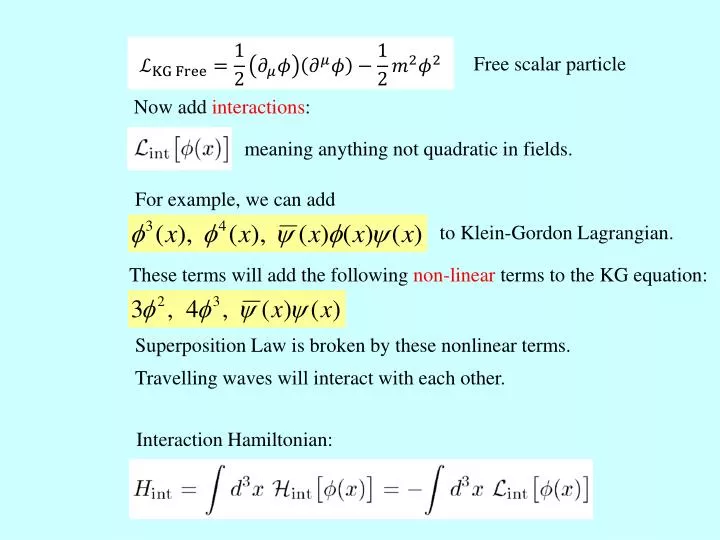
Free scalar particle Now add interactions: meaning anything not quadratic in fields. For example, we can add to Klein-Gordon Lagrangian. These terms will add the following non-linearterms to the KG equation: Superposition Law is broken by these nonlinear terms. Travelling waves will interact with each other. Interaction Hamiltonian:
量子力學的原則 狀態 波函數 運算子 物理量測量 有古典對應的物理量就將位置算子及動量算子代入同樣的數學形式: 測量期望值 狀態波函數滿足疊加定律,因此可視為向量, 所有的狀態波函數形成一個無限維向量空間,稱Hilbert Space。
狀態可視為向量,因此可以以抽象的向量符號來代表。狀態可視為向量,因此可以以抽象的向量符號來代表。 Dirac Notation 狀態 Ket Bra 測量 算子 與 內積 測量期望值 測量值確定的本徵態
Schrodinger Picture States evolve with time, but not the operators: It is the default choice in wave mechanics. 狀態 波函數 測量 算子 Evolution Operator: the operator to move states from to .
In quantum mechanics, only expectation values are observable. For the same evolving expectation value, we can instead ask operators to evolve. We move the time evolution to the operators: Now the states do not evolve. Heisenberg Picture How does the operator evolve? Heisenberg Equation The rate of change of operators equals their commutators with H.
In Schrodinger picture, field operators do not change with time, looking not Lorentz invariant. Fields operators in Heisenberg Picture are time dependent, more like relativistic classical fields. For KG field without interaction:
Combine the two equations The field operators in Heisenberg Picture satisfy KG Equation. The field operators with interaction satisfy the non-linear Euler Equation, for example
Interaction picture (Half way between Schrodinger and Heisenberg) There is a natural separation between free and interaction Hamiltonians: Move just the free H0 to operators. The rest of the evolution, that from the interaction H, stays with the state. States and Operators both evolve with time in interaction picture:
Evolution of Operators Operators evolve just like operators in the Heisenberg picture but with the full Hamiltonian replaced by the free Hamiltonian For field operators in the interaction picture: Field operators are free, as if there is no interaction! The Fourier expansion of a free field is still valid.
Evolution of States Hint Iis just the interaction Hamiltonian Hint in interaction picture! States evolve like in the Schrodinger picture but with full Hreplaced by Hint I. That means, the field operators in Hint Iare free.
Interaction Picture Operators evolve just like in the Heisenberg picture but with the full Hamiltonian replaced by the free Hamiltonian States evolve like in the Schrodinger picture but with the full Hamiltonian replaced by the interaction Hamiltonian.
The evolution of states in the interaction picture Define U the evolution operator of states. All the problems can be answered if we are able to calculate this operator is the state in the future t which evolved from a statein t0 is the state in the long future which evolves from a stateinthe long past. The amplitude for to appear as a state is their inner product: = The amplitude is the corresponding matrix element of the operator.
The transition amplitude for the decay of A: the amplitude of in the long future which evolves fromthe long past. The transition amplitude for the scattering of A: S operator is the key object in particle physics!
U has its own equation of motion: The evolution of states in the interaction picture is the evolution operator of states. Take time derivative on both sides and plug in the first Eq.:
Perturbation expansion of U and S Solve it by a perturbation expansion in small parameters in HI. To leading order:
To leading order, S matrix equals It is Lorentz invariant if the interaction Lagrangian is invariant.
Vertex In ABC model, every particle corresponds to a field: Add the following interaction term in the Lagrangian: The transition amplitude for A decay: can be computed as : To leading order:
The remaining numerical factor is: B C Momentum Conservation ig A
For a toy ABC model Three scalar particle with masses mA, mB ,mC 1 External Lines Internal Lines Lines for each kind of particle with appropriate masses. C -ig Vertex A B The configuration of the vertex determine the interaction of the model.
A B C interaction Lagrangian vertex Every field operator in the interaction corresponds to one leg in the vertex. Every field is a linear combination of a and a+ Every leg of a vertex can either annihilate or create a particle! This diagram is actually the combination of 8 diagrams!
A B C Interaction Lagrangian vertex The Interaction Lagrangian is integrated over the whole spacetime. Interaction could happen anywhere anytime. The amplitudes at various spacetime need to be added up. The integration yields a momentum conservation. In momentum space, the factor for a vertex is simply a constant.
Interaction Lagrangian Vertex Every field operator in the interaction corresponds to one leg in the vertex. Every leg of a vertex can either annihilate or create a particle!
Propagator Solve the evolution operator to the second order. HI is first order. The integration of two identical interaction Hamiltonian HI. The first HI is always later than the second HI
The integration of two identical interaction Hamiltonian HI. The first HI is always later than the second HI t’ and t’’ are just dummy notations and can be exchanged. t’’ We are integrating over the whole square but always keep the first H later in time than the second H. t’
t’’ This definition is Lorentz invariant! t’
This notation is so powerful, the whole series of operator U can be explicitly written: The whole series can be summed into an exponential:
Amplitude for scattering Fourier Transformation Propagator between x1 and x2 p2-p4 pour into C at x1 p1-p3 pour into C at x2
B(p3) B(p4) x1 C(p1-p3) x2 C A(p1) A(p2) A particle is created at x2 and later annihilated at x1. B(p4) B(p3) A(p1) A(p2)
B(p3) B(p4) x2 x1 C(p1-p3) x2 x1 C C A(p1) A(p2) A particle is created at x1 and later annihilated at x2. B(p4) B(p3) B(p4) B(p3) A(p1) A(p1) A(p2) A(p2)
B(p3) B(p4) x2 x1 C(p1-p3) x2 x1 C C A(p1) A(p2) B(p4) B(p3) B(p4) B(p3) A(p1) A(p1) A(p2) A(p2) This construction ensures causality of the process. It is actually the sum of two possible but exclusive processes. Again every Interaction is integrated over the whole spacetime. Interaction could happen anywhere anytime and amplitudes need superposition.
This propagator looks reasonable in coordinate space but difficult to calculate and the formula is cumbersome.
This doesn’t look explicitly Lorentz invariant. But by definition it should be! So an even more useful form is obtained by extending the integration to 4-momentum. And in the momentum space, it becomes extremely simple:
B(p3) B(p4) x2 x1 C(p1-p3) x2 x1 C C A(p1) A(p2) The Fourier Transform of the propagator is simple. B(p4) B(p3) B(p4) B(p3) A(p1) A(p1) A(p2) A(p2)
B(p3) B(p4) x2 x1 C(p1-p3) x2 x1 C C A(p1) A(p2) B(p4) B(p3) B(p4) B(p3) A(p1) A(p1) A(p2) A(p2)
For a toy ABC model Internal Lines Lines for each kind of particle with appropriate masses.
Every field either couple with another field to form a propagator or annihilate (create) external particles! Otherwise the amplitude will vanish when a operators hit vacuum!
For a toy ABC model Three scalar particle with masses mA, mB ,mC 1 External Lines Internal Lines Lines for each kind of particle with appropriate masses. C -ig Vertex A B The configuration of the vertex determine the interaction of the model.
Scalar Antiparticle Assuming that the field operator is a complex number field. The creation operator b+ in a complex KG field can create a different particle! The particle b+ create has the same mass but opposite charge. b+ create an antiparticle.
Complex KG field can either annihilate a particle or create an antiparticle! Its conjugate either annihilate an antiparticle or create a particle! The charge difference a field operator generates is always the same! So we can add an arrow of the charge flow to every leg that corresponds to a field operator in the vertex.
incoming particle or outgoing antiparticle incoming antiparticle or outgoing particle charge non-conserving interaction
incoming antiparticle or outgoing particle incoming particle or outgoing antiparticle charge conserving interaction
incoming antiparticle or outgoing particle incoming particle or outgoing antiparticle can either annihilate a particle or create an antiparticle! can either annihilate an antiparticle or create a particle!
U(1) Abelian Symmetry The Lagrangian is invariant under the field phase transformation invariant is not invariant U(1) symmetric interactions correspond to charge conserving vertices.
A If A,B,C become complex, they all carry charges! B C The interaction is invariant only if The vertex is charge conserving.