Download
1 / 19
200 likes | 461 Views
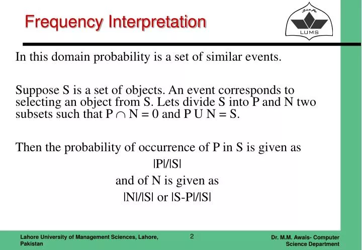
Frequency Interpretation. In this domain probability is a set of similar events. Suppose S is a set of objects. An event corresponds to selecting an object from S. Lets divide S into P and N two subsets such that P N = 0 and P U N = S.

E N D
Frequency Interpretation In this domain probability is a set of similar events. Suppose S is a set of objects. An event corresponds to selecting an object from S. Lets divide S into P and N two subsets such that P N = 0 and P U N = S. Then the probability of occurrence of P in S is given as |P|/|S| and of N is given as |N|/|S| or |S-P|/|S|
Subjective Interpretation A subjective probability is a probability expressing a person’s degree of belief in a proposition or the occurrence of an event. Well prepared students can have higher level of confidence in passing the exam. Other types of probability approaches can be used to enhance the interpretation of the subjective probability
Certainty Factors Certainty Factor theory is based on subjective Probability and is commonly used in Expert Systems to handle uncertainty. Lets define: MB=Measure of belief MD=Measure of Disbelief CF=Certainty Factor = MB-MD If CF is 1 the evidence for the hypothesis being true is 100% If the CF value is 0 the evidence is 0%. If CF approaches -1 the evidence of disbelief is 100%.
Algebra of CF CF reflects the confidence of the expert in the rule’s reliability. Typical Rule: IF A and B THEN C (And B are premise and D is conclusion) Algebra for the Premise: for premise P1, P2, ……, The CF values are calculated as follows: AND operator CF(P12)=CF(P1 and P2)=MIN(CF(P1),CF(P2)) CF(P12 and P3)=MIN(CF(P12) and P3)) and so on OR operator CF(P12)=CF(P1 or P2)=MAX(CF(P1),CF(P2)) CF(P12 or P3)=MAX(CF(P12) and P3)) and so on
Algebra Suppose the rule is IF (P1 and P2 ) or P3 THEN C1 and CF(P1)=0.6, CF(P2)=0.4, CF(P3)=0.2 For premise the combined CF will be CF(P)=MAX( MIN(CF(P1),CF(P2)), CF(P3)) Algebra for the Overall rule: CF(Rule)=CF(P)*CF(C1)
Combining Rules When two or more rules support the same conclusion CF(R1)+CF(R2) - CF(R1)*CF(R2) where all values are positive When two or more rules do not support the same conclusion CF(R1)+CF(R2) + CF(R1)*CF(R2) where all values are negative Otherwise [CF(R1)+CF(R2)]/[1-MIN(|CF(R1)|,|CF(R2|)]
Example: MYCIN IF the infection is primary_bacteria (0.6) AND the site of the culture is one of the sterile sites(0.5) AND the suspected portal of the entry is gastrointestinal tract (0.8) THEN there is suggestive evidence that infection is bacteriod (0.7) CF(P)=MIN(0.6,0.5,0.8)=0.5 CF(R)=0.5*0.7=0.35
Example 1: Suppose we have the following rule R1: if (P1 and P2 andP3) or (P4 and not P5 then C1 (0.7) and C2(-0.5) and the certainty factors of P1, P2, P3, P4, P5 are as follows: CF(P1) = 0.8,CF(P2) = 0.7,CF(P3) = 0.6,CF(P4) = 0.9,CF(P5) = -0.5, What are the certainty factors associated with conclusions C1 and C2 after using rule R1?
Example 1: Solution: For P1 and P2 and P3, the CF ismin(CF(P1), CF(P2), CF(P3)) = min(0.8, 0.7, 0.6) = 0.6. Call this CFA. For not P5, the CF is -CF(P5) = 0.5. For P4 and notP5, the CF is min(0.9, 0.5) = 0.5. Call this CFB. For (P1 and P2 and P3) or (P4 and notP), the CF is:max(CFA, CFB) = max(0.6, 0.5) = 0.6. Thus CF(C1) = 0.7 * 0.6 = 0.42and CF(C2) = -0.5 * 0.6 = -0.30
Example 2: The final answers to the previous question are CFR1(C1) = 0.42 and CFR1(C2) = -0.3. Suppose that we have, from another rule R2, the following certainty factors for C1 and C2: CFR2(C1) = 0.7, CFR2(C2) = -0.4 What are the certainty factors associated with C1 and C2 after combining the evidence from rules R1 and R2?
Example2: Solution: For C1, CF(C1) = CFR1(C1) + CFR2(C1) - CFR1(C1)*CFR2(C1)= 0.42 + 0.7 - 0.42*0.7 = 1.12 - 0.294 = 0.826. For C2, CF(C2) = CFR1(C2) + CFR2(C2) + CFR1(C2)*CFR2(C2)= -0.3 + -0.4 + (-0.3)*(-0.4) = -0.7 + 0.12 = -0.58
Modifying the CF values: If after getting new information the CF value is to be changed then CF(revised)=CF(old) + CF(new)*(1-CF(old)) What is 1-CF(old)? (the amount of doubt present in the old evidence)
Bayesian Approach: IF there is hypothesis H then the P(H) gives the probability of H being true. If a certain evidence (E) is present for the happening of H then the probability is given as P(H|E). This is referred as Conditional Probability, defined as: P(H|E) = P(H^E) / P(E) where P(H^E) is the probability that both H and E are true.
Gathering Information: Conditional Probability, may be obtained from experts. Example: we can know the probability of a heart attack given shooting pain in the arm from a doctor. (It is easier to obtain suitable data on people who had heart attack, than people who have had shooting pains) Thus we have Bayes’ Rule that says: P(H|E) = [P(E|H) * P(H) ] / P(E)
Independence What happens if more than one evidences are available?. The two evidences may or may not have any influence on each other if that’s the case then: P(E1^E2)=P(E1)*P(E2) (example: tossing a coin) But generally the evidences are not independent, thus conditional independence is used which is P(H|E1^E2^….) = [P(E1^E2...|H) * P(H) ] / P(E1^...) where P(E1^E2….) is the Joint Distribution of all the evidences
Independence What happens if more than one evidences are available?. The two evidences may or may not have any influence on each other if that’s the case then: P(E1^E2)=P(E1)*P(E2) (example: tossing a coin) But generally the evidences are not independent, thus conditional independence is used which is P(H|E1^E2^….) = [P(E1^E2...|H) * P(H) ] / P(E1^...) where P(E1^E2….) is the Joint Distribution of all the evidences
Likelihood Ratios Prior Odds O(H)=P(H) / 1-P(H) Posterior Odds O(H|E) = P(H|E) /1- P(H|E) Likelihood Ratio (Level of Sufficiency) LS= P(E | H) / P(E | ¬H) Using odds and the likelihood ratio definitions: O(H | E) = LS * O(H) Multiple Evidences: O(H|E1^E2…..) = (LS1*LS2*…..)*O(H)
Example Suppose we have obtained the following likelihood ratios LSs Measles LS Mumps LS spots 15 10 no spots 0.3 0.5 high temp. 4 5 no temp. 0.8 0.7 The prior odds for two diseases are 0.1 and 0.05 for measles and mumps. Calculate the posterior odds of the diseases for • spots and no temperature • no spots and temperature • no spots and no temperature
Example O(Measles|spots and no temp) = 0.1*15*0.8=1.2 O(Mumps|spots and no temp)=0.05*10*0.7=0.35