Download
1 / 29
300 likes | 452 Views
Dynamics of a Continuous Model for Flocking. Ed Ott in collaboration with Tom Antonsen Parvez Guzdar Nicholas Mecholsky. Dynamical Behavior in Observed Bird Flocks and Fish Schools. Our Objectives - Introduce a model and use it to investigate:. Flock equilibria Relaxation to equilibrium

E N D
Dynamics of a Continuous Model for Flocking Ed Ott in collaboration with Tom Antonsen Parvez Guzdar Nicholas Mecholsky
Our Objectives- Introduce a model and use it to investigate: • Flock equilibria • Relaxation to equilibrium • Stability of the flock • Response to an external stimulus, e.g. flight around a small obstacle: poster of Nick Mecholsky
Characteristics of Common Microscopic Models of Flocks • Nearby repulsion (to avoid collisions) • Large scale attraction (to form a flock) • Local relaxation of velocity orientations to a common direction • Nearly constant speed, v0
Continuum Model • Many models evolve the individual positions and velocities of a large number of discrete boids. • Another approach (the one used here) considers the limit in which the number of boids is large and a continuum description is applicable. • Let The number density of boids The macroscopic (locally averaged) boid velocity field
Governing Equations: Conservation of Boids: 1 Velocity Equation: 2 3 4
(1). Short range repulsion: This is a pressure type interaction that models the short range repulsive force between boids. The denominator prevents r from exceeding r* so that the boids do not get too close together.
(2). Long-range attraction: Here kr-1 represents a ‘screening length’ past which the interaction between boids at and becomes ineffective. In this case, satisfies: and U satisfies: These equations for u and U apply in 1D, 2D, and 3D.
(3). Velocity orientation relaxation term: Our choice for satisfies:
(4).Speed regulation term: This term brings all boids to a common speed v0. If |v| > v0 (|v| < v0 ), then this term decreases (increases) |v|. If , the speed |v| is clamped to v0.
Equilibrium We consider a one dimensional flock in which the flock density, in the frame moving with the flock, only depends on x. Additionally, v is independent of x and is constant in time (v0):
Equilibrium Solutions The equilibrium equations combine to give an energy like form where F depends on a dimensionless parameter a (defined below) and both r and x are made dimensionless by their respective physical parameters r* and kr
An Example and the density at x = 0 is determined to be
Solving the potential equation, we get The profile is symmetric about
Waves and Stability Equilibrium: Perturbations:
Basic Equation: where: and the notation signifies the operator
Long Wavelength Expansion Ordering Scheme:
Analysis: Inner product of equation for with annihilates higher order terms to give:
Comment: The eigenfunction from the analysis represents a small rigid x-displacement whose amplitude varies as exp(ikyy + ikzz).
Cylindrical Flock We have also done a similar analysis for a cylindrical flock with a long wavelength perturbation along the cylinder axis.
Numerical Analysis of Waves and Stability Linearized equations are a coupled system for dr, dvx, and dvy. Discretize these functions of position, and arrange as one large vector. Use a standard algorithm to determine eigenvalues and eigenvectors. The solutions give all three branches of eigenvalues and their respective eigenfunctions.
Preliminary Conclusions From Numerical Stability Code: • All eigenmodes are stable (damped). • For small k (wavelength >> layer width), the damping rate is much larger than the real frequency. • For higher k (wavelength ~ layer width), the real frequency becomes bigger than the damping rate.
Flock Obstacle Avoidance We consider the middle of a very large flock moving at a constant velocity in the positive x direction. The density of the boids is uniform in all directions. The obstacle is represented by a repulsive Gaussian hill
Solution using Linearized System Add the repulsive potential, linearize the original equations Fourier-Bessel transform in
Black = Lower Density, White = Higher Density