Download
1 / 12
120 likes | 219 Views
Correlation. We can often see the strength of the relationship between two quantitative variables in a scatterplot, but be careful. The two figures here are both scatterplots of the same data , on different scales. The second seems to be a stronger association…

E N D
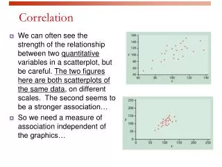
Correlation • We can often see the strength of the relationship between two quantitative variables in a scatterplot, but be careful. The two figures here are both scatterplots of the same data, on different scales. The second seems to be a stronger association… • So we need a measure of association independent of the graphics…
Use the correlation coefficient, r The correlation coefficient is a measure of the direction and strength of a linear relationship. It is calculated using the mean and the standard deviation of both the x and y variables. Correlation can only be used to describe quantitative variables. Categorical variables don’t have means and standard deviations.
The correlation coefficient r Time to swim: = 35, sx = 0.7 Pulse rate: = 140 sy = 9.5
You DON'T want to do this by hand. Make sure you learn how to use your calculator or the computer to find r. z for time z for pulse Part of the calculation involves finding z, the standardized score similar to the one we used when working with the normal distribution. Standardization: Allows us to compare correlations between data sets where variables are measured in different units or when variables are different. For instance, we might want to compare the correlation between [swim time and pulse], with the correlation between [swim time and breathing rate].
r = -0.75 r = -0.75 "Time to swim" is the explanatory variable here, and belongs on the x axis. However, in either plot r is the same (r=-0.75). r does not distinguish between x & y The correlation coefficient, r, treats x and y symmetrically
r = -0.75 z-score plot is the same for both plots r = -0.75 r has no unit of measure (unlike x and y) Changing the units of measure of variables does not change the correlation coefficient r, because we "standardize out" the units when getting z-scores. z for time z for pulse
r ranges from -1 to +1 r quantifies the strength and direction of a linear relationship between 2 quantitative variables. Strength: how closely the points follow a straight line. Direction: is positive when individuals with higher X values tend to have higher values of Y.
When variability in one or both variables decreases, the correlation coefficient gets stronger ( closer to +1 or -1).
Correlation coefficient r describes linear relationships No matter how strong the association, r should not be used to describe non-linear relationships - we have other methods… Note: You can sometimes transform a non-linear association to a linear form, for instance by taking the logarithm. You can then calculate a correlation using the transformed data.
Influential points Correlations are calculated using means and standard deviations, and thus are NOT resistant to outliers - try the Statistical Applet under Resources in the eBook on the Stats Portal… Just moving one point away from the general trend here decreases the correlation from -0.91 to -0.75
Go to the Stats Portal, under Resources, try Statistical Applets, and choose the Correlation and Regression one… put some points in the scatterplot, watch the value of r and see what happens when you put in an outlier or two… In this example, adding two outliers decreases r from 0.95 to 0.61.
Homework: • Read section 2.2, pay careful attention to the properties of the correlation coefficient, r • To explore how extreme outlying observations influence r, play around with the Statistical Applet on Correlation and Regression under Resources in the eBook on the Stats Portal… • Then, using the computer to draw the scatterplots and do the computations as needed, do problems #2.42 - 2.44, 2.47, 2.53, 2.55, 2.56, 2.60