Download
1 / 37
370 likes | 469 Views
On approximating a geometric prize-collecting traveling salesman problem with time windows. Reuven Bar-Yehuda – Technion IIT Guy Even – Tel Aviv Univ. Shimon (Moni) Shahar –Tel Aviv Univ. 1.5 hours. 4 hours. 2 hours. 2 hours. 2 hours. 1 hour. 1 hour. 1 hour.

E N D
On approximating a geometric prize-collecting traveling salesman problem with time windows Reuven Bar-Yehuda – Technion IIT Guy Even – Tel Aviv Univ. Shimon (Moni) Shahar –Tel Aviv Univ.
1.5 hours 4 hours 2 hours 2 hours 2 hours 1 hour 1 hour 1 hour Motivation – postman distributing packages 10:00-11:00 6:00-7:00 12:00-8:00 16:00-17:00 0.5 hour rest 17:00-18:00 7:00-5:00 7:00-6:00 leave office at 5:00 get back at 20:00 12:00-8:00
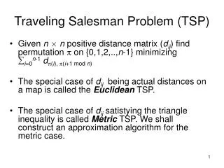
Prize-collecting TSP with time windows • A scheduling problem with locations. • Definition: • Sites in a metric space (e.g. the plane). • A time-interval for each site (release-time, deadline). • Moving agent with speed in [0,1]. • Goal: max #sites the agent visits on-time. • Extension: service-time per site.
Known results: scheduling with locations • Feasibility is NPC for points on a line [Tsitsiklis92]. • Polynomial algorithm for the case where all intervals are [0,ti] (using dynamic programming) [Tsitsiklis92 Khanna02] • Min makespan (completion time of last job): • 1.5-approx for points on a line with release times, processing times, and no deadlines [KNI98]. • 2-approx for points on a line, no deadlines, multiple agents (vehicles) [KN01]. • PTAS for trees with O(1) leaves, single & multiple agents [AS02].
t y x
t y x
t y x
t y x
t x
t x
t x
t x
speed = 1/slope Slope in [450, 1350] Chop intervals outside of visibility cone
After we rotate the view by 450, Slope of tour [0, 90]
Special case: zero length Longest monotone subsequence
Approach: Longest path on a DAG
Approach: Longest path on a DAG
Approach: Longest path on a DAG
Approach: Longest path on a DAG
t Approach works for any dimension: Longest path on a DAG y x
Longest path on a DAG t y x
Polynomial time algorithms: • If all interval times have zero length • If Max length ≤ k * Min Length Grid path: Opt in time Poly(n,2k) General: 2-approx in time Poly(n,2k) General: O(log k /loglogn) - approx • No assumptions: O(log(n)) - approximation
1 1 1 1 1 1 2 1 1 1 1 1 1 Grid path: |intervalgrid| k • Construct a DAG. V={(x,y): (x,y) R2} • Direct the grid up & right. • Assign edge weights (#intersecting intervals). • Find a longest path on the obtained DAG. k-apx
0 1 0 0 (2,3) 1 (2,2) Grid path: |intervalgrid| k • Construct a DAG • V = {(x,y),b1…bk: • (x,y) R2 and bi {0,1}} • Directed “right” edges • (x,y)0b2…bk(x+1,y)b2…bk0 • (x,y)0b2…bk(x+1,y)b2…bk1 (2,2)1001 (2,3)0010 • Directed “up” edges • (x,y)1b2…bk(x,y+1)b2…bk0 • (x,y)1b2…bk(x,y+1)b2…bk1 • Assign edge weights and • find longest path in the DAG
A 2-approx for length [1,2) • Construct a 2/4 square grid. • Each interval intersects • at most 8 grid lines. • Find optimal grid path (k=8). • Time complexity: • Poly(n) • Claim: (optimal) path P: grid paths P1 P2, s.t • P1 and P2 cover all intervals intersected by P
P P1 P2 (optimal) path P: grid paths P1, P2, s.t P1 and P2 cover all intervals intersected by P P: an optimal path P1: Upper grid path P2: Lower grid path
A 2-approx for length [1,2) 2log(Imax/Imin)- apxfor the general case
A 2-approx for length [1,k) 2log(Imax/Imin)/logk- apxfor the general case k=O(logn) time is Poly(n)
Recursive bisection Claim: separating vertical line (at most half the intervals lie strictly on each side).
Level 2 Level 2 2nd comb Recursive bisection (cont.) • A comb defines subset of intervals that intersect exactly one comb-tooth. • bisect recursively log(n) “combs” • comb Ci such that: Ci OPT contains at least OPT/log n intervals. Level 1
O(log(n)) Approximation • Partition the intervals into log n combs. • For each comb 2-apx. • 2log(n)- approximation.
Approximation for comb • Construct a DAG. i i+1 • Form a grid. • V = • set of horz segments k j • Set of edges: • (i, j) (i+1, k) • If j k. Edge weights is the number • Of new intersected intervals weight((i, j), (i+1, k))=4
Approx ratio = 2 • Decompose OPT into alternating sub-tours: • horizontal sub-tours inside a slice • vertical sub-tours between two comb teeth • Each “covered segment” must cross P1 or P2 P1 P2
Zigzags: source of hardness • special case: no zigzags between intervals Dynamic programming finds optimal tour (even if distances are asymmetric). • Extension: density = bound on number of zigzag between intervals.apx ratio=density (same dynamic programming)
Further research • Improve approximation ratio in 1-D. • Nothing known for 2-D.