The conditioned stimulus

1. The conditioned stimulus • Generalization: A range of stimuli varying on a particular dimension will produce responses in proportion to how similar they are to the trained CS. • The generalization gradient is the graph of the strength of the CR to stimuli varying above and below the CS.

2. A generalization gradient

3. Discrimination learning • If stimuli other than the CS are presented, but never paired with the US, the generalized responses to similar stimuli will diminish, so that the individual discriminates between CS and non-CS. • Examples of classically-conditioned discrimination learning abound in education: colors, shapes, letters...The color or shape or letter is CS, the teacher’s word for it is the US.

4. Results of discrimination learning Generalizationaround a light CS of 500nm Discriminationaround a light CS of 500nm 40 30 20 Eyeblinksper minute 10 0 470 480 490 500 510 520 530 Wavelength of light, nm (Color)

5. Long-term potentiation • A neural basis of learning • Strong stimulation of one of two connected neurons at time 1 increases the likelihood that a later weak stimulus from neuron 1 will trigger a response in neuron 2. • This potentiation of the connection lasts for several hours. • That may be the basis for classical conditioning.

6. LTP and classical conditioning • A US neuron has a strong input to a UR neuron, while a CS neuron has a weak input to the same UR neuron. • If the US neuron is active while the CS neuron is active, it may potentiate the connection between the CS neuron and the UR neuron.

7. Synaptic plasticity: Neural Learning • NMDA (N-methyl-D-aspartate) receptors and AMPA (a-amino-3-hydroxy-5-methyl-4-isoxazole propionate) receptors for the neurotransmitter glutamate, a general excitatory neurotransmitter. • If the US neuron triggers AMPA action within the UR neuron at the same time that the CS neuron is weakly stimulating the UR neuron, then the two actions may add together to make the CS-UR/CR connection more sensitive to future CS stimulation. • This action is thought to increase NMDA receptor activity.

8. 0 The nature of the CR • Two theories: • 1. CR = UR (cf. stimulus substitution) • 2. CR prepares for UR • What do the data say? • The CR is always different from the UR. • Sometimes the CR differs from the UR only in magnitude, duration, or latency. • But sometimes, the CR is opposite to the UR: Relaxation and slowed heart rate as a CR to a CS for shock, but agitation and increased heart rate as a UR to the actual shock US. (cf. Siegel, 1975)

9. Opponent Process Theory • Opponent processes are bodily reactions opposite to the effect of a US, in order to preserve physiological balance. • If a CS is conditioned to a US, the opponent process rather than the UR becomes the CR. • Wagner (1981) argued that opponent processes are conditioned as CRs only for URs which provoke compensatory reactions—biphasic responses, but not for monophasic URs: SOP.

10. Applications of SOP • Drug tolerance • CS (setting for drug taking) + US (drug)  CR (tolerance) • US (drug) without CS (setting)  Overdose • Spousal boredom • CS (setting: Usual routine) + US (spouse)  CR (boredom) • US (spouse) without CS (new setting)  Excitement

11. Contiguity theory • The S-S and S-R theories we have studied operate on the associationist principle of contiguity: eg. Research on CS-US intervals. • Delay conditioning • Trace conditioning and the optimal interval • Simultaneous conditioning (<450 msec) • Backward conditioning

12. What kind of contingency produces learning? • The curious conclusion is that perfect contiguity impairs association. How can that be? • Recall sensory preconditioning. • Simultaneous conditioning allows association between stimuli, but does not produce a CR.

13. Is there another view? • Contingency theory • A competing view is called contingency: differential prediction of the US by the CS, not mere co-occurrence. • Recall simultaneous and backward conditioning. • In a contingent relationship, p(US | CS) > p(US | not-CS)

14. Consider three key studies Rescorla, (1966)/(1968) Garcia & Koelling (1966) Kamin (1969)

15. Rescorla and contingency learning • The greater the differential contingency, the greater the learning. • In Lieberman and Sniffy, the suppression ratio is B/(A+B), the response rate in the presence of the CS divided by the total number of responses, and so the lower the suppression ratio, the greater the learned fear of CS. • For Rescorla, the suppression ratio is (A - P)/(A + P) • A is the response rate in the Absence of the CS • P is the response rate in the Presence of the CS • If A = P, there is no suppression, and the ratio = 0 • If A > P, there is suppression, expressed in the ratio. • Thus, the higher the ratio, the greater the suppression, and the greater the learning.

16. Contiguity or contingency: Rescorla (1968) • Notice that the greater the difference between the pUS|CS and the pUS|CS, the greater the suppression ratio: Contingency.

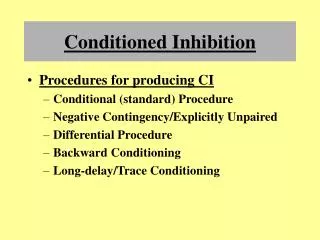
17. Occasion setting and conditioned inhibition • Conditioned inhibition: Summation paradigm • Separately condition CS+ to US and CS- to not-US • Test CS+ and CS- together • Amount of reduction of CR shows strength of CS- • Conditioned inhibition: Retardation paradigm • First condition CS- to not-US • Then, keeping CS-, try to condition CS+ to US • Amount of retardation of conditioning shows strength of CS- • Occasion setting • Clocks and kisses

18. Preparedness and associative bias: Garcia & Koelling (1966) • Observation of bait shyness but not place shyness • A shock US conditions better to light/tone CS than to taste CS • A nausea-inducing drug or radiation US conditions better to taste CS than to light/tone CS • Contiguity is clearly insufficient for learning. • Possible conclusion: Associations are reasonable inferences

19. Stimulus combinations 1: Blocking • Overshadowing • Kamin (1968): Informativeness, redundancy, and blocking Group 1: CS1(Noise) + CS2(Light)  US(Shock) (eight trials) Group 2: CS1  US (sixteen trials) CS1 + CS2  US (eight trials) Group difference? Blocking

20. Stimulus combinations 2: Unblocking Kamin (1969): Unblocking (repeated trials) Phase 1: CS1  US (1mA shock) CS1 + CS2  US (1mA shock) Test CS2: Almost no evidence of conditioning Phase 2: CS1 + CS2  US (4mA shock) Test CS2 CR (measured as CER) Thus, the change in the US unblocks the previously blocked CS2.

21. Stimulus combinations 3: Surprise! Kamin’s explanation: When the rat is surprised by the US, it searches its memory for a CS to use as a predictor in the future. In blocking situations, there is no surprise, so no conditioning to CS2. In unblocking situations, the rat is surprised by the change in the US, so conditions to CS2. Note the crucial role of memory in Kamin’s explanation.

22. Stimulus combinations 4: Good news! Rescorla(1966) had found that negative differential contingency (pUS|CS<pUS|not-CS) also produced conditioning, but it was inhibitory. Similarly, in a Kamin-like experiment, Dickinson, Hall, and Mackintosh (1976) showed that if a stimulus compound (CS1 + CS2) signaled a reduction in the US, unblocking occurred.

23. Rescorla-Wagner theory • The theory has an equation with three parts: • V, the amount of learning acquired • a , the rate of learning sponsored by the CS • b , the rate of learning sponsored by the US • l , the maximum amount of learning that can happen to the particular US. • Together, DVn = ab ( l - Vn) • Or as Lieberman has it, DVn = c (Vmax - Vn) The equation is applied once for each learning trial, to see how much learning will happen on each trial.

24. Example of Rescorla-Wagner computations • DV = ab ( l - Vn) • If ab = .20 and l = 100, work through 4 trials: • Trial 1: .20 ( 100 - 0) = 20 • Trial 2: .20 ( 100 - 20) = 16 • Trial 3: .20 ( 100 - 36) = 12.8 • Trial 4: .20 ( 100 - 48.8) = 10.24 • Note the diminishing returns with repeated trials. Will learning ever stop? • The learning decreases as the CS becomes less surprising.

25. Another example • DVn = ab ( l - Vn) • If ab = .10 and l = 200, work through 5 trials: • Trial 1: .10 ( 200 - 0) = 20 • Trial 2: .10 ( 200 - 20) = 18 • Trial 3: .10 ( 200 - 38) = 16.2 • Trial 4: .10 ( 200 - 54.2) = 14.58 • Trial 5: .10 ( 200 - 68.78) = 13.12 • In a relative sense, learning is happening more slowly here.

26. A learning curve from Rescorla-Wagner theory

27. Rescorla-Wagner and compound stimuli • Competitive learning: The total learning available, l , must be shared by each stimulus in a compound. Thus, the amount of learning to each stimulus is less in a compound than if that stimulus is alone. • VAB = VA + VB • Rescorla-Wagner predicts extinction, contingency, overshadowing, blocking, and conditioned inhibition accurately.

28. R-W compounds: • Trial 1: DVA = DVB = .20(100 – 0) = 20 Trial 2: DVA = DVB = .20(100 – 40) = 12 instead of DVA = .20(100 – 20) = 16 • Note that stimulus compounds share the associative strength.

29. Overshadowing • Trial 1: DVA = .40(100 – 0) = 40 DVB = .10(100 – 0) = 10 • Trial 2: DVA = .40(100 – 50) = 20 DVB = .10(100 – 50) = 5

30. Blocking • If, after 16 trials, VA = 100, then DVB = .20(100 – 100) = 0 • But if the US changes, such that l = 200, DVB = .20(200 – 100) = 20: Unblocking.

31. Conditioned inhibition: Safety signals and the overexpectation effect • If learning has proceeded to the point that VA = 100 and VA + VB = 0, then what must VB equal? • Rescorla-Wagner nicely predicts conditioned inhibition (Rescorla, 1970): • Pair a tone with shock and a light with shock • Follow with 12 trials pairing tone+light with the same shock • Test tone and light separately for CER • Result: Reduced CER to tone and to light: Overexpectation.

32. Problems with Rescorla-Wagner • 1. CS preexposure produces slower conditioning to CS later, a phenomenon known initially (Lubow & Moore, 1959) as latent inhibition. For example, displaying the letters of the alphabet around the classroom before they are learned is CS preexposure. • The CS preexposure effect is not predicted by Rescorla-Wagner, unless you assume that preexposure lowers the learning rate (ab) by lowering salience.

33. 2. Configural cue learning • Rescorla-Wagner predicts that in a compound stimulus situation, the learning to the compound CS1 + CS2 will be the sum of the learning to each CS. • But Pearce (1994) and others show that in stimulus compound situations, there is not individual cue learning: • A + B but not A or B; • A or B but not A + B; • [A+C and B+D] but not [A + C or B + D] • Compare with perceptual organization: Do you see letters, or words, or phrases in this sentence?

34. 3. Associative bias or preparedness • As we have seen, some CS-US combinations have different ab values • R-W does not show how to find them.

35. Occasion setting • Recall that an occasion setter is an additional CS that indicates that another CS will (or won’t) be followed by the US. • An occasion setter does not directly associate with the US. • If the occasion setter is presented repeatedly without US, its effect as an occasion setter for responding to the CS is not extinguished, or even reduced.

36. Another remarkable thing: • If the occasion setter is inhibitory with a CS, and is then paired alone (excitatory conditioning) with the US, it remains an inhibitory occasion setter with the CS. • The occasion setter may serve to facilitate the connection between CS and US, without becoming connected itself.

37. Connectionism: A Neural model • Learning may involve forming patterns of synaptic connections. • ABCD --> CR1, ie US1 • ABCF --> CR2, ie US2 • The rule for connection formation is the delta rule, based on Rescorla-Wagner for stimulus compound situations. • CSs are inputs; USs are outputs. • These are neural networks.

38. Applications of classical conditioning • Classroom structure • Make salient what is to be learned • Eliminate redundant CSs • Establish differential contingency • Extinction by exposure • Flooding • Counterconditioning in desensitization • Aversion therapy • Consider preparedness, generalization issues

39. So, what is learned in classical conditioning? • A teleological cognition • Tolman (1932) and expectation • CS  US: Expectation for the future • Fits with CR as preparation for US, eg. SOP • Fits with choice in US devaluation studies (Colwill & Motzkin, 1994): rats know which US will be presented. • CS1  Sucrose solution US • CS2  Food pellets • Then devalue sucrose US: Lowered approaches to CS1 but not to CS2. • Stimulus substitution • Pavlov: The CS becomes the US • Autoshaping fits this view: Jenkins & Moore, 1973

40. A Two-system hypothesis • Stimulus substitution fits an associative system. • Expectations fit a cognitive system. • Paralleled in brain structures • Paleocortex/allocortex and neocortex/isocortex • Two pathways to the amygdala • Direct from the senses: Fast, associative • Indirect via the cortex: Slow, cognitive • Timberlake, Wahl, & King (1982): Timing of a rolling ball CS fit the two-system hypothesis • But how do we predict which system will activate?

41. Conditioning without awareness • Unconscious associations • Ohman & Soares (1998) • Advertising as conditioning • Attractive model • Eating while watching commercials • Music on commercials • Celebrity endorsements • Is causal learning like classical conditioning?

42. The Little Albert studies (Watson & Rayner, 1920)

43. Generalization in Little Albert (Watson & Rayner, 1920) • In this clip, Little Albert, who has already been taught to fear the rat, now shows at least discomfort in the presence of a rabbit. Watson’s interpretation was that the fear of the rat generalized to the rabbit.