Download
1 / 65
650 likes | 787 Views
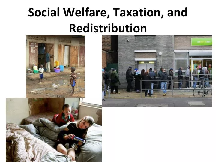
Social Welfare, Taxation, and Redistribution. V Equity and Distribution. Introduction. The Second Theorem of Welfare Economics has strong policy implications The policy analysis begins by assuming a social planner can make judgements over allocations of utility

E N D
V Equity and Distribution Introduction • The Second Theorem of Welfare Economics has strong policy implications • The policy analysis begins by assuming a social planner can make judgements over allocations of utility • The only intervention is a lump-sum redistribution of endowments to ensure that consumers have the required incomes
V Equity and Distribution Social Optimality • The first issue is the selection of one of the Pareto-efficient allocations from the contract curve • There are a number of ways this can be done • Voting over the alternative allocations or for the election of a body (a ‘government’) to make the choice • Consumers could agree for the allocation to be chosen at random or they might hold unanimous views • There may be a benevolent social planner who has preferences over the alternative allocations based on the utility levels of the consumers
V Equity and Distribution Social Optimality • The social planner assesses the welfare of society by aggregating individual consumers’ welfares • The function that undertakes this aggregation is a Bergson-Samuelson social welfare function • Given a pair of welfare levels {U1, U2} the social welfare function is W(U1, U2) • The social welfare function embodies the equity considerations of the social planner in the shape of the social indifference curves
V Equity and Distribution Social Optimality • The utilitarian social welfare function (no concern for equity) is defined by W =U1 + U2 • The Rawlsian social welfare function (maximal concern for equity) is defined by W =min{U1, U2} Utilitarian Intermediate Rawlsian Figure 13.2 Social indifference curves
V Equity and Distribution Lump-Sum Taxes • Lump-sum taxes enable decentralization • A transfer or tax is lump-sum if a consumer cannot affect the size of the transfer by changing behaviour • Making every consumer pay the same fixed amount is an example of a lump-sum tax system • The value of lump-sum taxes rests on their imposition being costless • There are two aspects to being costless • Lump-sum taxes cause no distortions in choice • Implementing them uses no resources
V Equity and Distribution Lump-Sum Taxes • The primary concern is optimal lump-sum taxes • Taxes are optimal when the resulting equilibrium is socially optimal • To calculate optimal lump-sum taxes the social planner must predict the equilibrium for all income levels • This requires knowledge of the consumers’ preferences and the value of each consumer’s endowment • These economic characteristics are private information • They are known only to the individual consumers
V Equity and Distribution Lump-Sum Taxes • Optimal lump-sum taxes must depend on characteristics • As the characteristics are not observable the social planner must: • Either rely on consumers to honestly report them • Or the characteristics must be inferred from actions • In the latter case taxes are affected by choice of action and so are not lump-sum • Consumers will only report characteristics honestly if given an incentive to do so
V Equity and Distribution Lump-Sum Taxes • It may not be possible to make optimal lump-sum taxes incentive compatible • Let a consumer’s endowment be determined by IQ • If the level of tax is inversely related to IQ an IQ test would not be cheated • If taxes were positively related to IQ then testing would be manipulated by the high IQ consumers intentionally doing poorly • In the second case taxes are not incentive compatible • There is potential for misrevelation of characteristics
V Equity and Distribution Impossibility of Lump-Sum Taxes • To implement the Second Theorem optimal lump-sum taxes must be used • The taxes may be costly to collect and will not be incentive compatible • The theorem shows what could be possible not what is possible • It is the impracticality of optimal lump-sum taxes the motivates studying other forms of taxation • All other taxes are distortionary but can be implemented
Redistribution In-Kind • Governments frequently provide goods at less than cost • This is a form of redistribution • Standard arguments show a cash transfer of the same value to be preferable • But: • Making a program universal ensures political support • Targeted cash for education would receive less support • Redistribution is limited through self-selection • The high-ability eventually choose the allocation designed for the low-ability • In-kind transfers provide less incentive for the high-ability to mimic the low-ability • Consider the limited incentive for the healthy to claim health care provision
Inequality and Poverty • A social welfare function allows equity to be addressed • But information restricts the applicability of the concept • There are other measures of equity • These may not be ideal but are applicable • Inequality and poverty measures provide an alternative perspective on distribution • Inequality refers to an unequal distribution of income (or wealth) • Poverty refers to the existence of very low incomes
Income • A first step to measuring inequality or poverty is to measure income • Income is a flow so is measured over a given time period • For tax purposes income is the receipt of resources • This works but is backward-looking • Economic choices are made in advance of income being received • A forward-looking measure is necessary
Equivalence Scales • Households differ in size and age distribution • A large family need more income to reach a given level of welfare than a small family • Demographic variables include the number of adults, the number of children, and the ages of family members • Observed household incomes must be adjusted to take demographic variables into account • Equivalence scales are a method for making incomes comparable across households
Equivalence Scales • A minimum needs scale uses the cost of a basic bundle of goods and services • The bundle varies with household demographics • Tab. 14.1 reports some implementations • The Rowntree scale sees $60 for a single person as equivalent to $100 for a couple Table 14.1 Minimum needs equivalence scales
Equivalence Scales • The Engel scale hypothesises that the expenditure share of food is proportional to welfare • In Fig. 14.1 incomes M1and M2lead to the same share s for demographics d1and d2 • These incomes are equivalent • This can be extended to the iso-prop method for a basket of goods Expenditure share of food Income Figure 14.1 Construction of Engel scale
V Equity and Distribution Inequality Measurement • Inequality is easy to recognize but harder to quantify • A quantitative measure is require to compare inequality across time or across countries • An inequality measure is a single number that captures the inequality in a distribution • Measures can be constructed using standard statistical indexes or constructed from explicit welfare assumptions • These approaches are not unrelated
V Equity and Distribution Inequality Measurement • There are H households labelled h = 1,…,H • Incomes are ordered so M1 ≤ M2 ≤ … ≤ MH • The mean income is • An inequality measure assigns a number between 0 and 1 to the distribution {M1,…, MH} • A value of 0 represents complete equality • A value of 1 represents complete inequality (one person receives all income)
V Equity and Distribution Inequality Measurement • The simplest inequality measure is the range defined by R = (MH – M1)/m • Division by m ensures R is a relative index (independent of units for measuring income) • R does not take account of the intermediate incomes between MHand M1 • The relative mean deviation, D, defined by D = Sh|m – Mh|/2[H – 1]m, takes account of all incomes • D is insensitive to transfers between households on the same side of the mean income level
V Equity and Distribution Inequality Measurement • The way a measure should react to transfers is summarized in the Pigou-Dalton Principle • Definition 14.1 (Pigou-Dalton Principle of Transfers) The inequality index must decrease if there is a transfer of income from a richer household to a poorer household that preserves the ranking of the two households in the income distribution and leaves total income unchanged • A measure that satisfies this is sensitive to transfers • Neither R nor D satisfy this principle
V Equity and Distribution Inequality Measurement • The coefficient of variationC = s/m, where s2 = Sh[Mh – m]2/H, is sensitive to transfers • For C the effect of a transfer does not depend on the income levels of the households involved but only the difference in incomes between the households • But an argument can be made that a given transfer should have a larger effect at low incomes • This observation suggests that satisfaction of the Pigou-Dalton Principle may not be the only property required
V Equity and Distribution Inequality Measurement • The Lorenz curve is a graphical representation of an income distribution • The population is arranged in order of income and the proportion of population is graphed against proportion of income • If there is inequality the Lorenz curve is below the diagonal • Fig. 14.4 plots a typical Lorenz curve Figure 14.4 Construction of a Lorenz curve
V Equity and Distribution Inequality Measurement • A transfer of income from poor to rich moves the Lorenz curve away from the diagonal • Distributions can be ranked if the Lorenz curves do not cross • In Fig. 14.5 distribution Ahas less inequality than Bwhen the curves do not cross • Lorenz curves provide a partial ordering A A B B A more equal than B A and B incomparable Figure 14.5 Lorenz curves as an incomplete ranking
V Equity and Distribution Inequality Measurement • The Gini coefficient is frequently used in applied research • The Gini considers all possible pairs of incomes, selects the lowest from each pair, and then averages • G is defined by G = 1 – (1/H2m)SiSjmin{Mi, Mj}
V Equity and Distribution Inequality Measurement • The Gini provides a complete ranking • It also satisfies the Pigou-Dalton Principle and the response to a transfer depends on locations of the households in the distribution • If an amount of income G is transferred from household i to household j where Mi < Mj then DG =(2/H2m)[j – i]G> 0 • The ranking by Lorenz curves can be related to the Gini
V Equity and Distribution Inequality Measurement • The value of the Gini is equal to twice the area between the Lorenz curve and the main diagonal • This is shown in Fig. 14.6 • The value of Gis twice the grey area • The Gini provides a ranking even when Lorenz curves cross Figure 14.6 Relating Gini to Lorenz
V Equity and Distribution Inequality Measurement • The Pigou-Dalton Principle can be interpreted as a welfare criterion • Looking for any “desirable” property of an inequality measure implies normative reasoning • Inequality measures and social welfare can be linked • Let social welfare be measured by the function W = W(M1,…, MH) • W(M1,…, MH) is assumed to be symmetric and concave
V Equity and Distribution Inequality Measurement • Theorem 14.2 (Atkinson) Consider two distributions of income with the same mean. If the Lorenz curves for these distributions do not cross, every symmetric and concave social welfare function will assign a higher level of welfare to the distribution whose Lorenz curve is closest to the main diagonal • The proof of this theorem is based on moving from the outer to the inner Lorenz curve • This is achieved by transferring income from richer to poorer households • The assumptions of symmetry and concavity imply these transfers raise social welfare
V Equity and Distribution Inequality Measurement • The converse of the theorem is that if the Lorenz curves cross two welfare functions can be found that rank them differently • Hence the Lorenz curves provides the most complete ranking possible without further restrictions on social welfare • Any complete ranking must imply restrictions on social welfare • This idea can be developed into the construction of the welfare functions implicit in statistical measures
V Equity and Distribution Inequality Measurement • Fig. 14.7 depicts the social indifference curves for the Gini • A redistribution of income leaves G unchanged if it leaves [[2H-1]M1 + …+ MH] constant • For a population of two households this reduces to 3M1+M2 • This gives the curves plotted (Note the roles change when M1>M2) Figure 14.7 Gini social welfare
V Equity and Distribution Inequality Measurement • All statistical measures of inequality embody implicit welfare assumptions • These assumptions may not be acceptable • An alternative approach is to begin with a welfare function and construct the implied inequality measure • This is the Atkinson approach to inequality measurement which makes the welfare assumptions explicit
V Equity and Distribution Inequality Measurement • Assume that the welfare function is utilitarian with W = ShU(Mh) • And that the utility function satisfies U′(M) > 0, U′′(M) < 0 • Define the equally distributed equivalent income, MEDE, by ShU(Mh) = HU(MEDE) • The Atkinson measure of inequality is given by A = 1 –MEDE/m
V Equity and Distribution Inequality Measurement • The construction of MEDEisshown in Fig. 143.8 • The income distribution is {M1, M2} • The concavity of utility implies MEDE< m • This guarantees that 0 ≤ A ≤ 1 • MEDEfalls if M2is increased relative to M1 Income of household 2 Social indifference curve Income of household 1 Figure 14.8 Equally distributed equivalent income
V Equity and Distribution Inequality Measurement • Application of the Atkinson measure typically assume that U(M) = M1-e/(1 - e), e ≠ 1 U(M) = log(M) , e = 1 • The welfare judgement is contained in the choice of e • The utility function becomes more concave as e increases • This represents a greater social concern for equity
V Equity and Distribution Inequality Measurement • Tab. 14.2 summarizes an OECD study • Contrast of measures before and after tax show tax system is redistributive • Contrast over time shows an increase in inequality • The measures are fairly consistent Table 14.2 Inequality before and after taxes and transfers
V Equity and Distribution Poverty • Poverty is the possession of fewer resources than necessary to attain an acceptable standard of living • Poverty can be defined in absolute or relative terms • Absolute poverty assumes a fixed minimum level of consumption that constitutes poverty independent of time or place • Relative poverty is defined in terms of a given society and given time • The poverty line delineates who is in poverty
V Equity and Distribution Poverty • A poverty line can be defined for both absolute and relative concepts of poverty • The US uses a package of minimum needs to define the poverty line • This implies a concept of absolute poverty • The UK defines the poverty line as a proportion of the minimum benefit level • Hence a relative poverty concept is implied • The switch from poverty to non-poverty across a single line is a strong assumption
V Equity and Distribution Poverty Percentage population living on less than 1 dollar day 2007-2008
V Equity and Distribution Poverty • Let the poverty line be fixed at z • The income gap for household h is given by gh = z – Mh • Given an income distribution {M1,…, MH} the number of households in poverty is q where Mq≤z but Mq+1> z • The simplest poverty measure is the headcount ratio E = q/H • This measure is easy to compute but insensitive to incomes below the poverty line
V Equity and Distribution Poverty • The aggregate poverty gap sums the income gaps of the households in poverty • This measure is defined by V = gh • V shows the income required to alleviate poverty • It is incentive to transfers of income below the poverty line unless one household is taken out of poverty • It is not sensitive to the number in poverty
V Equity and Distribution Poverty • The income gap ratio, I, takes into account the number in poverty I = (1/z)gh/q • Division by z ensures 0 ≤I≤ 1 • But the measure I can show increased poverty when a transfer raises a household out of poverty • Changing from the distribution {1, 9, 20, 40, 50} to {1, 10, 20, 40, 50} with z = 10 raises I from 0.5 to 0.9
V Equity and Distribution Poverty • The discussion suggests a poverty measure should possess the following properties: • It should not be affected by transfers of income between households above the poverty line • It should increase if a poor household becomes worse off • The measure should be anonymous • It should rise after a regressive transfer • Two further properties are: • More weight should be given to the poorest • It should reduce to the headcount if the poor have identical incomes
V Equity and Distribution Poverty • All these conditions are satisfied by the Sen measure S = E[I + [1 – I]Gpq/(q+1)] • Gpis the Gini for incomes below the poverty line • By combining information on the number in poverty (q), the income shortfall (I), and distribution, Gp, this measure avoids the shortcomings of individual measures • This illustrates the value of deriving a measure that satisfies a set of specified conditions (often called axioms)
V Equity and Distribution Poverty • Tab. 14.4 summarizes an OECD study • A range of measures and poverty lines are used • The focus is on the change in poverty over time • The income gap can be inconsistent with other measures • Poverty has increased in some countries Table 14.4 Evolution of poverty (% change in poverty measure)
V Equity and Distribution Poverty Poverty is defined as an income which most people would regard as being too low to buy the necessities
V Equity and Distribution Unequal Opportunities • Sources of inequality of outcome can be morally acceptable or unacceptable • Unequal outcomes that are a consequences of factors for which individuals are responsible (“effort”) should not be compensated • Inequality from “circumstances” should be compensated for • Circumstances can include family background, race, gender, place of birth
V Equity and Distribution Unequal Opportunities • Equality of opportunity exists when no set of circumstances is preferred to another set by all individuals • Let s and s’ be two circumstances and F(x|s) the probability of obtaining an outcome less than or equal to x • Inequality of opportunity in terms of first-order stochastic dominance hold when F(x|s)≤F(x|s’)
V Equity and Distribution Unequal Opportunities • An alternative condition is to use second-order stochastic dominance • This holds is the expected value for s is less than the mean outcome for s’