Download

1 / 17
200 likes | 465 Views
Programming For Nuclear Engineers Lecture 14 MATLAB Applications. 1- The 360° Pendulum 2- Heat Equation 3- A SIMULINK Solution. 1- The 360° Pendulum Normally we think of a pendulum as a weight suspended by a flexible string or

E N D
Programming For Nuclear Engineers Lecture 14MATLAB Applications
1- The 360° Pendulum 2- Heat Equation 3- A SIMULINK Solution
1- The 360° Pendulum Normally we think of a pendulum as a weight suspended by a flexible string or cable, so that it may swing back and forth. Another type of pendulum consists of a weight attached by a light (but inflexible) rod to an axle, so that it can swing through larger angles, even making a 3600 rotation if given enough velocity . Though it is not precisely correct in practice, we often assume that the magnitude of the frictional forces that eventually slow the pendulum to a halt is proportional to the velocity of the pendulum. Assume also that the length of the pendulum is 1 meter, the weight at the end of the Pendulum has mass 1 kg, and the coefficient of friction is 0.5. In that case, the equations of motion for the pendulum are:
Where t represents time in seconds, x represents the angle of the pendulum from the vertical in radians (so that x = 0 is the rest position), y represents the velocity of the pendulum in radians per second. Here is a phase portrait of the solution with initial position x(0) = 0 and initial velocity y(0) = 5. This is a graph of x versus y as a function of t, on the time interval 0 ≤ t ≤ 20. g = inline(’[x(2); -0.5*x(2) - 9.81*sin(x(1))]’, ’t’, ’x’); [t, xa] = ode45(g, [0 20], [0 5]); plot(xa(:, 1), xa(:, 2))
Recall that the x coordinate corresponds to the angle of the pendulum and the y coordinate corresponds to its velocity. Starting at (0, 5), as t increases we follow the curve as it spirals clockwise toward (0, 0). The angle oscillates back and forth, but with each swing it gets smaller until the pendulum is virtually at rest by the time t = 20. Meanwhile the velocity oscillates as well, taking its maximum value during each oscillation when the pendulum is in the middle of its swing (the angle is near zero) and crossing zero when the pendulum is at the end of its swing.
Next we increase the initial velocity to 10. [t, xa] = ode45(g, [0 20], [0 10]); plot(xa(:, 1), xa(:, 2))
2- Heat Equation We will use MATLAB to numerically solve the heat equation (also known as the diffusion equation), a partial differential equation that describes many physical processes including conductive heat flow or the diffusion of an impurity in a motionless fluid. You can picture the process of diffusion as a drop of dye spreading in a glass of water. The dye consists of a large number of individual particles, each of which repeatedly bounces off of the surrounding water molecules, following an essentially random path. There are so many dye particles that their individual random motions form an essentially deterministic overall pattern as the dye spreads evenly in all directions (we ignore here the possible effect of gravity). In a similar way, you can imagine heat energy spreading through random interactions of nearby particles.
In a three-dimensional medium, the heat equation is: Here u is a function of t, x, y, and z that represents the temperature, or concentration of impurity in the case of diffusion, at time t at position (x, y, z) in the medium. The constant k depends on the materials involved; it is called the thermal conductivity in the case of heat flow and the diffusion coefficient in the case of diffusion. To simplify matters, let us assume that the medium is instead one-dimensional. This could represent diffusion in a thin water-filled tube or heat flow in a thin insulated rod or wire. Then the partial differential equation becomes:
Where u(x, t) is the temperature at time t a distance x along the wire. To solve this partial differential equation we need both initial conditions of the form u(x, 0) = f (x), where f (x) gives the temperature distribution in the wire at time 0, and boundary conditions at the endpoints of the wire; call them x = a and x = b. We choose so-called Dirichletboundary conditions u(a, t) = Ta and u(b, t) = Tb , which correspond to the temperature being held steady at values Ta and Tb at the two endpoints. The following M-file, named heat.m, give an iteration procedure for the problem:
function u = heat(k, x, t, init, bdry) % solve the 1D heat equation on the rectangle described by % vectors x and t with u(x, t(1)) = init and Dirichlet % boundary conditions % u(x(1), t) = bdry(1), u(x(end), t) = bdry(2). J = length(x); N = length(t); dx = mean(diff(x)); dt = mean(diff(t)); s = k*dt/dxˆ2; u = zeros(N,J); u(1, :) = init; for n = 1:N-1 u(n+1, 2:J-1) = s*(u(n, 3:J) + u(n, 1:J-2)) +... (1 - 2*s)*u(n, 2:J-1); u(n+1, 1) = bdry(1); u(n+1, J) = bdry(2); end
The function heat takes as inputs the value of k, vectors of t and x values, a vector init of initial values (which is assumed to have the same length as x), and a vector bdry containing a pair of boundary values. Its output is a matrix of u values. Notice that since indices of arrays in MATLAB must start at 1, not 0, we have deviated slightly from our earlier notation by letting n=1 represent the initial time and j=1 represent the left endpoint. Notice also that in the first line following the for statement, we compute an entire row of u, except for the first and last values, in one line; each term is a vector of length J-2, with the index j increased by 1 in the term u(n,3:J) and decreased by 1 in the term u(n,1:J-2). Let’s use the M-file above to solve the one-dimensional heat equation with k = 2 on the interval −5 ≤ x ≤ 5 from time 0 to time 4, using boundary temperatures 15 and 25, and initial temperature distribution of 15 for x < 0 and 25 for x > 0.
We must choose values for ∆t and ∆x; let’s try ∆t = 0.1 and ∆ x = 0.5, so that there are 41 values of t ranging from 0 to 4 and 21 values of x ranging from −5 to 5. tvals = linspace(0, 4, 41); xvals = linspace(-5, 5, 21); init = 20 + 5*sign(xvals); uvals = heat(2, xvals, tvals, init, [15 25]); surf(xvals, tvals, uvals) xlabel x; ylabel t; zlabel u Here we used surf to show the entire solution u(x, t). The output is clearly unrealistic; notice the scale on the u axis!
The solution to the problem above is thus to reduce the time step ∆t ; for instance, if we cut it in half: tvals = linspace(0, 4, 81); uvals = heat(2, xvals, tvals, init, [15 25]); surf(xvals, tvals, uvals) xlabel x; ylabel t; zlabel u This looks much better! As time increases, the temperature distribution seems to approach a linear function of x. Indeed u(x, t) = 20 + x is the limiting “steady state” for this problem; it satisfies the boundary conditions and it yields 0 on both sides of the partial differential equation.
3- A SIMULINK Solution We can also solve the heat equation using SIMULINK. SIMULINK solves the model using MATLAB’s ODE solver, ode45. To illustrate how to do this, let’s take the same example we started with, the case where k = 2 on the interval −5 ≤ x ≤ 5 from time 0 to time 4, using boundary temperatures 15 and 25, and initial temperature distribution of 15 for x < 0 and 25 for x > 0.
Note that one needs to specify the initial conditions for u as Block Parameters for the Integrator block, and that in the Block Parameters dialog box for the Gain block, one needs to set the multiplication type to “Matrix”. The output from the model is displayed in the Scope block in the form of graphs of the various entries of u as functions of t, but it’s more useful to save the output to the MATLAB Workspace and then plot it with surf. (It is left for you) .