Download
1 / 37
370 likes | 377 Views
2. Neurons and Conductance-Based Models. Fundamentals of Computational Neuroscience, T. P . Trappenberg , 2002. Lecture Notes on Brain and Computation Byoung-Tak Zhang Biointelligence Laboratory School of Computer Science and Engineering

E N D
2. Neurons and Conductance-Based Models Fundamentals of Computational Neuroscience, T. P . Trappenberg, 2002. Lecture Notes on Brain and Computation Byoung-Tak Zhang Biointelligence Laboratory School of Computer Science and Engineering Graduate Programs in Cognitive Science, Brain Science and Bioinformatics Brain-Mind-Behavior Concentration Program Seoul National University E-mail: btzhang@bi.snu.ac.kr This material is available online at http://bi.snu.ac.kr/
2.1 Modeling biological neurons • The networks of neuron-like elements • The heart of many information-processing abilities of brain • The working of single neurons • Information transmission • Simplified versions of the real neurons • Make computations with large numbers of neurons tractable • Enable certain emergent properties in networks • Nodes • The sophisticated computational abilities of neurons • The computational approaches used to describe single neurons
2.2.1 Structural properties (1) Fig. 2.1 (A) Schematic neuron that is similar in appearance to pyramidal cells in the neocortex. The components outlined in the drawing are, however, typical for major neuron types.
2.2.1 Structural properties (2) • Fig. 2.1 (B-E) Examples of morphologies of different neurons. • (B) Pyramidal cell from the motor cortex • (C) Granule neuron from olfactory bulb • (D) Spiny neuron from the caudate nucleus • (E) Golgi-stained Purkinje cell from the cerebellum.
2.2.2 Information-processing mechanisms • Neurons can receive signals from many other neurons • Synapses (contact site) • Presynaptic (from axon) • Postsynaptic (to dendrite or cell body) • Signal = action potential • Electronic pulse
2.2.3 Membrane potential • Membrane potential • The difference between the electric potential within the cell and its surrounding
2.2.4 Ion channels (1) • The permeability of the membrane to certain ions is achieved by ion channels Fig. 2.2 Schematic illustrations of different types of ion channels. (A) Leakage channels are always open. (B) Neurotransmitter-gated ion channel that opens when a neurotransmitter molecule binds to the channel protein, which in turn changes the shape of the channel protein so that specific ions can pass through. (C) The opening of voltage-gated ion channels depends on the membrane potential. This is indicated by a little wire inside the neurons and a grounding wire outside the neuron. Such ion channels can in addition be neurotransmitter-gated (not shown in this figure). (D) Ion pumps are ion channels that transport ions against the concentration gradients. (E) Some neurotransmitters bind to receptor molecules which triggers a whole cascade of chemical reactions in neurons which produce secondary messengers which in turn can influence ion channels
2.2.4 Ion channels (2) • Major ion channels • Pump: use energy • Channel: use difference of ions concentration
2.2.4 Ion channels (3) • Resting potential
2.3 Basic synaptic mechanisms • Signal transduction within the cell is mediated by electrical potentials. • Electrical synapse or gap-junctions • Chemical synapse • Synaptic plasticity 2.3.1 Chemical synapses and neurotransmitters • neurotransmitters stored in synaptic vesicles • glutamate (Glu) • gamma-aminobutyric acid (GABA) • Dopamine (DA) • acetylcholine (ACh) • synaptic cleft (a small gap of only a few micrometers) • Receptor (channel) and Postsynaptic potential (PSP) Fig. 2.3 (A) Schematic illustration of chemical synapses and (B) an electron microscope photo of a synaptic terminal.
2.3.2 Excitatory and inhibitory synapses • Different types of neurotransmitters • Excitatory synapse • PSP: depolarization • Neurotransmitters trigger the increase of the membrane potential • Neurotransmitter: Glu, ACh • Inhibitory synapse • PSP: hyperpolarization • Neurotransmitters trigger the decrease of the membrane potential • Neurotransmitter: GABA • Non-standard synapses • Influence ion channels in an indirect way • Modulation
2.3.3 The time-course of postsynaptic potentials • Excitatory postsynaptic potential (EPSP) resulting from non-NMDA receptors • w: amplitude factor • strength of EPSP or efficiency of the synapse • f(t)=t·exp(-t): α-function • functional form of a PSP • Inhibitory postsynaptic potential (IPSP) resulting from non-NMDA receptors • EPSP resulting from NMDA receptor (2.1) Fig. 2.4 Examples of an EPSP (solid line) and IPSP (dashed line) as modeled by an α-function after the synaptic delay. The dotted lines represent two examples of the difference of two exponential functions with different amplitudes. Note that the time scale is variable and not meant to fit experimental data in the illustration. Indeed, NMDA synapses are often much slower than non-NMDA synapses, often showing their maximal value long after the peak in the effect of the non-NMDA synapses. (2.2)
2.3.4 Superposition of PSP • Electrical potentials have the physical property • They superimpose as the sum of individual potentials. • Linear superposition of synaptic input • Nonlinear voltage-current relationship • Nonlinear interaction • Divisive • Shunting inhibition
2.4 The generation of action potentials Fig. 2.5 Typical form of an action potential, redrawn from an oscilloscope picture of Hodgkin and Huxley. Fig. 2.6 Schematic illustration o the minimal mechanisms necessary for the generation of a spike. The resting potential of a cell is maintained by a leakage channel through which potassium ions can flow as a result of concentration differences between the inside of the cell and the surrounding fluid. A voltage-gated sodium channel allows the influx of positively charged sodium ions and thereby the depolarization of the cell. After a short time the sodium channel is blocked and a voltage-gated potassium channel opens. This results in a hyperpolarization of the cell. Finally, the hyperpolarization causes the inactivation of the voltage-gated channels and a return to the resting potential.
2.4.3 Hodgkin-Huxley equations (1) • Quantified the process of spike generation • Input Current • Electric conductance • Membrane potential relative to the resting potential • Equilibrium potential • K+, Na+ conductance dependent • n, The activation of the K channel • m, The activation of the Na channel • h, The inactivation of the Na channel (2.3) Fig. 2.7 A Circuit representation of the Hodgkin-Huxley model. This circuit includes a capacitor on which the membrane potential can b e measured and three resistors together with their own battery modeling the ion channels; two are voltage-dependent and one is static. (2.4) (2.5)
2.4.3 Hodgkin-Huxley equations (2) • n, m, h have the same form of first-order differential-equation • x should be substituted by each of the variables n, m and h (2.6) Fig. 2.8 (A) The equilibrium functions and (B) time constants for the three variables n, m, and h in the Hodgkin-Huxley model with parameters used to model the gain axon of the squid.
2.4.3 Hodgkin-Huxley equations (3) Fig. 2.7 A Circuit representation of the Hodgkin-Huxley model. This circuit includes a capacitor on which the membrane potential can b e measured and three resistors together with their own battery modeling the ion channels; two are voltage-dependent and one is static. • Hodgkin-Huxley model • C, capacitance • I(t), external current • Three ionic currents (2.7) (2.8) (2.9) (2.10)
2.4.4 Numerical integration • A Hodgkin-Huxley neuron responds with constant firing to a constant external current. • The dependence of the firing rate with the external current (nonlinear curve). (dashed line: noise added) Fig. 2.9 (A) A Hodgkin-Huxley neuron responds with constant firing to a constant external current of Iext= 10. (B) The dependence of the firing rate with the strength of the external current shows a sharp onset of firing around Icext = 6 (solid line). High-frequency noise in the current has the tendency to ‘linearize’ these response characteristics (dashed line).
2.4.5 Refractory period • Absolute refractory period • The inactivation of the sodium channel makes it impossible to initiate another action potential for about 1ms. • Limiting the firing rates of neurons to a maximum of about 1000Hz • Relative refractory period • Due to the hyperpolarizing action potential it is relatively difficult to initiate another spike during this time period. • Reduced the firing frequency of neurons even further
2.5 Dendritic trees, the propagation of action potentials, and compartmental models • Axons with active membranes able to generate action potential • But, dendirtes are a bit more like passive conductors • The long cable • Cable theory • Compartmental models Fig. 2.10 Short cylindrical compartments describing small equipotential pieces of a passive dendrite or small pieces of a active dendrite or axon when including the necessary ion channels. (A) Chains and (B) branches determine the boundary conditions of each compartment. (C) The topology of single neurons can be reconstructed with compartments, and such models can be simulated using numerical integration techniques.
2.5.1 Cable theory (1) • Cable equation : the spatial-temporal variation of an electric potential • The potential of the cable at each location of the cable, • the physical properties of the cable and has the dimensions of Ωcm, • Ex) cylindrical cable of diameter d, • The specific resistance of the membrane, • The specific intracellular resistance of the cable, (2.11) (2.12)
2.5.1 Cable theory (2) • The time constant • The resistance of the membrane, • The capacitance, the capacitance per unit area, • Stable configuration • Semi-infinite cable • Nonlinear cable equation, include voltage-dependent ion channels as in the Hodgkin-Huxley equation (2.13) (2.14) (2.15) (2.16)
2.5.2 Physical shape of neurons • The physical shape of neurons • Simple homogeneous linear cableis to divide the cable into small pieces, compartment. • Each compartment is governed by a cable equation for a finite cable • The boundary conditions (2.17)
2.5.3 Neuron simulators • Ex) Neuron, Genesis Fig. 2.11 Example of the NEURON simulation environment. The example shows a simulation with a reconstructed pyramidal cell, in which a short current pulse was injected at t = 1 ms at the location of the dendrite indicated by the dot and the cursor in the window on the left.
2.6 Above and beyond the Hodgkin-Huxley neuron: fatigue, bursting, simplifications (1) • Simplification of the Hodgkin-Huxley model • The time constant is so small for all values of . • The rate of inactivation of the Na+ channel is approximately reciprocal to the opening of the K+ channel. • Neocortical neurons often show no inactivation of the fast Na+ channel. • The recovery of the membrane potential (2.18) (2.19)
2.6 Above and beyond the Hodgkin-Huxley neuron: fatigue, bursting, simplifications (2) • Extensions of the Hodgkin-Huxley model • Ca2+ channel, a dynamic gating variable T. • Slow hyperpolarizing current , Ca2+-mediated K+ channel, a dynamic gating variable H. (2.20) (2.24) (2.21) (2.25) (2.22) (2.26) (2.23)
2.6 Above and beyond the Hodgkin-Huxley neuron: fatigue, bursting, simplifications (3) • Simulation of the Wilson model Fig. 2.12 Simulated spike train of the Wilson model. The upper graph simulates fast spiking neurons (FS) typical of inhibitory neurons in the mammalian neocortex (τR = 1.5ms, gT = 0.25, gH = 0). The middle graph models regular spiking neurons (RS) with longer spikes (τR = 4.2ms, gT = 0.1). The slow calcium-mediated potassium channel (gH = 5) is responsible for the slow adaptation in the spike frequency. The lower graph demonstrate that even more complex behavior, typical of mammalian neocortical neurons, is incorporated in the Wilson model. The parameters (τR = 4.2ms, gT = 2.25, gH = 9.5) result I a typical bursting behavior, including a typical after-depolarizing potential (ADP).
Fig. 2.12 Simulated spike train of the Wilson model. The upper graph simulates fast spiking neurons (FS) typical of inhibitory neurons in the mammalian neocortex (τR = 1.5ms, gT = 0.25, gH = 0). The middle graph models regular spiking neurons (RS) with longer spikes (τR = 4.2ms, gT = 0.1). The slow calcium-mediated potassium channel (gH = 5) is responsible for the slow adaptation in the spike frequency. The lower graph demonstrate that even more complex behavior, typical of mammalian neocortical neurons, is incorporated in the Wilson model. The parameters (τR = 4.2ms, gT = 2.25, gH = 9.5) result I a typical bursting behavior, including a typical after-depolarizing potential (ADP).
Conclusion • Neurons utilize a variety of specialized biochemical mechanisms for information processing transmission • Membrane potential, ion channel • Action potential, neurotransmitter • Propagation, refractory period • Conductance-based models • Hodgkin-Huxley equation • Compartmental models • Cable theory • Neuron simulators • Neuron, Genesis