Decision Procedures for Data Structures

1. Decision Procedures for Data Structures Thomas Wies TexPoint fonts used in EMF. Read the TexPoint manual before you delete this box.: AAAAAAAAA

2. Outline Part I - Combining Theories with Shared Sets with RuzicaPiskac and Viktor Kuncak (FroCoS ‘09) Part II - Deciding Functional Lists with Sublist Sets with Marco Muñiz and Viktor Kuncak

3. Fragment of Insertion into Tree root size: right 4 3 left p left right data left tmp data data data e

4. Generated Verification Condition next0*(root0,n)  x {data0(v) | next0*(root0,v)} next=next0[n:=root0] data=data0[n:=x]  |{data(v) . next*(n,v)}| = |{data0(v) . next0*(root0,v)}| + 1 “The number of stored objects has increased by one.” • Expressing this VC requires a rich logic • transitive closure * (in lists and also in trees) • unconstraint functions (data, data0) • cardinality operator on sets | ... | • Is there a decidable logic containing all this?

5. Outline Part I - Combining Theories with Shared Sets Combination via Reduction BAPA-reducible Theories

6. Decomposing the Formula Consider a (simpler) formula |{data(x). next*(root,x)}|=k+1 Introduce fresh variables denoting sets:A = {x. next*(root,x)} B = {y.  x. data(x,y) xA}|B|=k+1 1) WS2S 2) C2 3) BAPA Good news: conjuncts are in decidable fragments Bad news: conjuncts share more than just equality(they share set variables and set operations) Next: explain these decidable fragments

7. f2 f1 f1 f2 f1 f2 WS2S: Monadic 2nd Order Logic Weak Monadic 2nd-order Logic of 2 Successors F ::= x=f1(y) | x=f2(y) | xS | ST | 9S.F | F1Æ F2 | :F - quantification is over finite sets of positions in a tree- transitive closure encoded using set quantification Decision procedure using tree automata (e.g. MONA)

8. C2 : Two-Variable Logic w/ Counting • Two-Variable Logic with Counting • F ::= P(v1,...,vn) | F1Æ F2 | :F | 9countvi.F • whereP : is a predicate symbol • vi : is one of the two variable names x,y • count : is =k, k, or k for nonnegative constants k • We can write (9kvi.F) as |{vi.F}|k • We can define 9,8 and axiomatize total functions: 8x9=1y.R(x,y) • Decidable sat. and fin-sat. (1997), NEXPTIME even for binary-encoded k: Pratt-Hartman ‘05

9. BAPA (Kuncak et al. CADE’05):Boolean Algebra with Presburger Arithmetic S ::= V | S1[ S2 | S1Å S2 | S1n S2T ::= k | C |T1 + T2 | T1 – T2 | C¢T | |S|A ::= S1 = S2 | S1µ S2 | T1 = T2 | T1 < T2F ::= A | F1Æ F2 | F1Ç F2 | :F |9S.F | 9k.F • BAPA decidable in alternating time (Kuncaket al. JAR’06), QFBAPA decidable in NP (Kuncaket al. CADE’07) • Also decidable: qf fragment of multisets w/ cardinalities • (Piskac, KuncakVMCAI’08,CAV’08,CSL’08) • New: role of BAPA in combination of theories sharing sets

10. Combining Theories by Reduction • Satisfiability problem expressed in HOL: • (all free symbols existentially quantified) next,data,k,root. 9 A,B.A = {x. next*(root,x)} B = {y.  x. data(x,y) xA}|B|=k+1 • We assume formulas share only: • - set variables (sets of uninterpretedelems) • - individual variables, as a special case - {x} 1) WS2S 2) C2 3) BAPA

11. Combining Theories by Reduction Satisfiability problem expressed in HOL, after moving fragment-specific quantifiers A,B. next,root. A = {x. next*(root,x)} data. B = {y.  x. data(x,y) xA}k. |B|=k+1 FWS2S FBAPA FC2 Extend decision procedures for fragments into projection procedures that reduce each conjunct to a decidable shared theory applies 9 to all non-set symbols

12. Combining Theories by Reduction Satisfiability problem expressed in HOL, after moving fragment-specific quantifiers A,B.next,root. A = {x. next*(root,x)} data. B = {y.  x. data(x,y) xA}k. |B|=k+1 Check satisfiability of conjunction of projections FWS2S FBAPA FC2  A,B. FWS2SÆ FC2Æ FBAPA Conjunction of projections satisfiableso is original formula

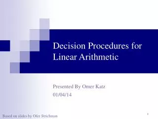
13. Fragment of Insertion into Tree size: 4 right left p left right data left tmp data data data e

14. Reduction of VC for insertAt Conjunction of projections unsatisfiable  so is original formula

15. Outline Part I - Combining Theories with Shared Sets Combination via Reduction BAPA-reducible Theories

16. Decision Procedure for Combination • Separate formula into WS2S, C2, BAPA parts • For each part, compute projection onto set vars • Check satisfiability of conjunction of projections • BAPA is natural target for the reduction

17. Amalgamation of Models:The Disjoint Case model for F model for G ? model for F Æ G Cardinalities of the models coincide model for F Æ G

18. Amalgamation of Models:The Set-Sharing Case model for F model for G Cardinalities of all Venn regions over shared sets coincide model for F Æ G

19. BAPA-Reducibility Definition: Theory is BAPA-reducibleiffthe projections of formulas onto set variables are expressible in BAPA.

20. BAPA-Reducible Theories

21. BAPA-Reducible Theories • MSOL over trees • 2-variable logic w/ counting • BSR • Qf-multisets with cardinalities • BAPA • Algebraic data types w/ generalized folds [Suter, Kuncak ‘10] • Sets with relation and function images [Yessenov, Piskac, Kuncak ‘10] • Ordered collections [Piskac, Suter, Kuncak ‘10] • Functional lists with sublist sets [TW, Muñiz, Kuncak ‘10] [TW, Piskac, Kuncak ‘09]

22. Outline Part I - Combining Theories with Shared Sets Part II - Deciding Functional Lists with Sublist Sets

23. Dropping n Elements from a List def drop(n, xs) returning (zs) { if (n · 0) xs elsexs match { case nil ) nil case cons(x, ys) ) drop(n-1, ys) } } ensuring (zs¹xsÆ (n ¸ 0 Æ length(xs) ¸ n ! length(zs) = length(xs) – n)) xs = cons(d1, cons(d2, …cons(dn, zs)…))

24. Generated Verification Condition Xs={vs. vs¹xs} ÆYs={vs. vs¹xs} ÆZs={vs. vs¹xs} Æ n > 0 Æxs nil Æ cons(x,ys)=xsÆzs¹ysÆ (n-1¸0 Æ|Ys| ¸ n !|Zs|= |Ys| - (n-1)) !zs¹xsÆ (n ¸ 0Æ|Xs| ¸ n + 1 !|Zs| = |Xs| – n) n > 0 Æxs nil Æ cons(x,ys)=xsÆzs¹ysÆ (n-1¸0 Æ length(ys)¸n-1 ! length(zs)=length(ys)-(n-1)) !zs¹xsÆ (n ¸ 0 Æ length(xs) ¸ n ! length(zs) = length(xs) – n) Express length in terms of cardinalities of sublist sets length(xs) = |{vs. vs¹xs}| - 1 • Set-sharing combination of the theories of • Functional lists with sublist sets and • BAPA

25. Outline Part I - Combining Theories with Shared Sets Part II - Deciding Functional Lists with Sublist Sets Deciding Functional Lists with Sublists Extension with Sublist Sets

26. Functional Lists with Sublists (FLS) TH ::= vH | head(TL) TL ::= vL | nil | cons(TH,TL) | tail(TL) | TLu TL A ::= TL = TL | TH = TH | TL¹TL F ::= A| F Æ F | F Ç F | :F

27. Canonical Model of FLS … … Term algebra generated by nil, cons and constants a, b, c, … x ¹ y iff tail*(y,x) … cons(a,cons(b,nil)) cons(b,cons(b,nil)) … … tail tail … cons(c,nil) cons(a,nil) cons(b,nil) tail ¹ tail tail nil tail

28. Idea of Decision Procedure for FLS Reduce satisfiability in the canonical model to satisfiability in the finite substructures (eliminate cons) Give a first-order axiomatizationof the theory of the finite substructures Show that the axiomatization is a local theory extension [Sofronie-Stokkermans ’05] of the empty theory Use hierarchical reasoning to reduce satisfiability in FLS to satisfiabiliy in BSR Complexity: NP Implementation: e.g., via [Jacobs ‘09]

29. Elimination of cons Rewrite all occurrences of cons in a formula F: F[cons(s,t)]  F[x] Æ x  nil Æ head(x) = s Æ tail(x) = t Resulting formula F’ is equisatisfiable to F. What is more: F’ is satisfiable in the canonical model iff F’ is satisifiable in one of the finite substructures

30. Axioms of the Theory Pure: Nil: Refl: Trans: AntiSym: Total: UnfoldR: UnfoldL: GCS1: GCS2: GCS3: head(x)=head(y) Æ tail(x)=tail(y) ! x=y Ç x=nil Ç y=nil nil ¹ x x ¹ x x ¹ y Æ y ¹ z ! x ¹ z x ¹ y Æ y ¹ x ! x = y y ¹ x Æ z ¹ x ! y ¹ z Ç z ¹ y tail(x) ¹ x x ¹ y ! x = y Ç x ¹ tail(y) x u y ¹ x x u y ¹ y z ¹ x Æ z ¹ y ! z ¹ x u y Finite models of the axioms are isomorphic to the finite substructures.

31. Local Theory Extension Base theory: empty theory Base symbols: ¹ and constant symbols Extension theory: axioms K from previous slide Extension symbols: head, tail, u Locality condition: for every (finite) set of clauses G K[ G ² ? iffK[G] [ G ²?

32. Completion of Partial Models h h t t h h h t h t t t h h t t h t h nil Extend partial interpretations of extension symbols Start from finite total model for ¹-axioms

33. Outline Part I - Combining Theories with Shared Sets Part II - Deciding Functional Lists with Sublist Sets Deciding Functional Lists with Sublists Extension with Sublist Sets

34. Extension with Sets of Sublists • Extend the logic with the sublist set operator ¾(x): • ¾(x) = {y | y ¹ x} • and consider formulas of the form: • s1 = ¾(x1) Æ … Æsn = ¾(xn) ÆF(x1,…,xn) • set-sharing combination with BAPA enables • reasoning about list length • limited forms of universal quantification

35. BAPA-Reduction for FLS BAPA-Reduction For any FLS formula F(x1,…,xn) there exists a BAPA formula G(s1,…,sn) such that 9x1, …, xn, ¹, u, cons, tail, head, nil. s1 = ¾(x1) Æ … Æsn = ¾(xn) ÆF(x1,…,xn) is equivalent to G(s1,…,sn) Every FLS formula F is equivalent to a finite disjunction of partial models ) enumerate partial models using hierarchical reasoning and compute BAPA-reduction for each partial model

36. BAPA-Reduction for Partial Models Sx,y = (¾(x) n ¾(y))n {x} x Sx,y h h y t t Generate set constraint: ¾(x) = {x} [Sx,y[¾(y) Æ ¾(y) = {y} [¾(z) Æ … ¾(nil) = {nil} Æ disjoint(x, y, z, Sx,y, Sz,nil, …) h z Sz,nil h nil

37. Dropping n Elements from a List def drop(n, xs) returning (zs) { if (n · 0) xs elsexs match { case nil ) nil case cons(x, ys) ) drop(n-1, ys) } } ensuring (zs¹xsÆ (n ¸ 0 Æ length(xs) ¸ n ! length(zs) = length(xs) – n)) xs = cons(d1, cons(d2, …cons(dn, zs)…))

38. Reduction of VC for drop Shared sets: Xs, Ys, Zs FLS Fragment: Xs = ¾(xs) Æ Ys = ¾(ys) Æ Zs = ¾(zs) Æ xs nil Æ cons(y,zs) = xsÆzs¹ys Projection onto Xs, Ys, Zs: Zs µ Ys Æ Ys µ Xs Æ |Xs| > 1 Æ |Xs| = |Ys| + 1 BAPA Fragment: n > 0 Æ (n - 1 ¸ 0 Æ |Ys| ¸ n ! |Zs| = |Ys| - (n – 1) ) Æ n ¸ 0 Æ |Xs| ¸ n + 1 Æ |Zs|  |Xs| - n Projection onto Xs, Ys, Zs: |Xs|  |Ys| + 1 Conjunction of projections unsatisfiable so is original formula

39. Extension with List Content Extend the logic with the list content operator ¿(x): ¿(x) = head[¾{x} n {nil}] where head[S] = {head(x) | x 2 S} Image constraints containing terms head[S] can be eliminated using ideas from [Yessenov, Piskac, Kuncak ’10]. We obtain a decidable theory for reasoning about lists, sublists, sublist sets, list length, and list content.

40. Related Work on Combination Nelson-Oppen, 1980 – disjoint theories reduces to equality logic (finite # of formulas) Tinelli, Ringeissen, 2003 – general non-disjoint case we consider the particular case of sets Ghilardi – sharing locally finite theoriescardinality on sets needed, not locally finite Fontaine – gentle and shiny theories (BSR, …) Sofronie-Stockkermans – local theory extensions Ruess, Klaedtke – WS2S + cardinality (no C2, etc.) Reduction procedures to SAT (UCLID) we reduce to (QF)BAPA (NP-complete)reduction QFBAPA  QFPA  SAT non-trivial

41. Related Work on Functional Lists Oppen ‘78, Barret, Shikanian, Tinelli ‘07 – term algebras no sublist relation, no sets Venkataraman ‘87 – term algebras with subterm relation no sets, no practical implementations Sofronie-Stokkermans ‘09 – local theory extensions for term algebras with certain recursive functions Makanin ‘79, Jaffar ’90, Plandowski ’04 – word equations more expressive than sublists, higher complexity, no sets Bouajjani, Dargoi, Enea, Sighireanu ’09, Lahiri, Qadeer ’08 – trans. closure logics for function graphs axiom Pure requires new decision procedures

42. Summary Presented new combination technique for theories sharing sets by reduction to a common shared theory (BAPA). Identified an expressive decidable set-sharing combination of theories by extending their decision procedures to BAPA-reductions 1) WS2S, 2) C2,3) BSR, 4) BAPA, 5)qf-multisets 6) ADTs w/ generalized folds 7) sets w/ rel. images 8) ordered collections 9) FLS2 Resulting theory is useful for automated verification of complex properties of data structure implementations.

43. 0 0 0 0 0 0 0 0 10 0 1 10 0 1 10 0 1 10 0 1 0 0 0 0 0 0 AB BAPA-reduction for WS1S WS1S formula for a regular language F = ((A Æ:B)(B Æ:A))*(:B Æ:A)* Formulas are interpreted over finite words Symbols in alphabet correspond to (:A Æ:B),(A Æ:B),(:A Æ B),(AÆB) Model of formula F 00 10 01 11

44. BAPA-reduction for WS1S WS1S formula for a regular language F = ((A Æ:B)(B Æ:A))*(:B Æ:A)* Model of formula F A,B denote sets of positions in the word w. , , , denote Venn regions over A,B Parikh image gives card.s of Venn regions Parikh(w) = {  7,  4,  4,  0} } w 0 0 0 0 0 0 0 0 10 0 1 10 0 1 10 0 1 10 0 1 0 0 0 0 0 0 AB 00 10 01 11 00 10 01 11

45. BAPA-reduction for WS1S Decision procedure for sat. of WS1S: - construct finite word automaton A from F - check emptiness of L(A) Parikh 1966: Parikh image of a regular language is semilinear and effectively computable from the finite automaton Construct BAPA formula from Parikh image of the reg. lang.

46. BAPA-reduction for WS1S WS1S formula for a regular language F = ((A Æ:B)(B Æ:A))*(:B Æ:A)* Parikh image of the models of F: Parikh(F) = {(q,p,p,0) | q,p ¸ 0} BAPA formula for projection of F onto A,B: |A Å Bc| = |AcÅ B| Æ |A Å B| = 0 00 10 01 11

47. Combining Logics and Verifiers Bohne infers loop invariants of the form: B(S1,…,Sn) = Univ where B(S1,…,Sn) is a Boolean algebra expr. over sets S1,…,Sn defined in the individual theories