Download

1 / 74
740 likes | 850 Views
Decision Procedures for Linear Arithmetic. Presented By Omer Katz 01/04/14. Based on slides by Ofer Strichman. Agenda. DPLL-T (a very short reminder) What is Linear Arithmetic and why is it needed Decision procedures for Decision procedures for A few preprocessing improvement steps

E N D
Decision Procedures for Linear Arithmetic Presented By Omer Katz 01/04/14 Based on slides by OferStrichman
Agenda • DPLL-T (a very short reminder) • What is Linear Arithmetic and why is it needed • Decision procedures for • Decision procedures for • A few preprocessing improvement steps • Given enough time: • Difference logic • Delayed Theory Combination • Improvement on Nelson-Oppen • Not related to Linear Arithmetic
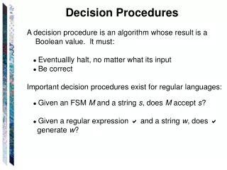
Reminder: DPLL-T • Our goal is to solve SMT problems with formulas from a theory T • DPLL-T is the most common approach • Based on the DPLL algorithm for SAT problems • Combines a decision procedure for the theory T
Linear Arithmetic • Theory grammar: • Can be defined over Rational () or Integers () • Example:
Why is it needed? Given the following C code: The following assembly can be generated:
Why is it needed? • A possible optimization: • Read the value of a[j] only once • Need to verify that loop won’t change a[j] • Can be encoded as Linear Arithmetic problem • If no solution is found, optimization is safe
Decision Procedures for • Gaussian’s elimination • Fourier-Motzkin • Simplex
Gaussian’s elimination • A simple method for solving a set of equalities • Less suitable for inequalities • Given a linear system Ax = b A x = b
Gaussian’s elimination • Manipulate A|b to an upper-triangular form • Then, solve backwards from the k’s row according to:
Gaussian elimination - example And now… x3 = -1, x2 = 3, x1 = 1 problem solved.
Fourier-Motzkin Elimination • Earliest method for solving linear inequalities • Given linear non-strict inequalities: • Pick a variable and eliminate it • Continue until all variables but one are eliminated • If problem included equalities, eliminate by assignment
A system of conjoined linear inequalities Fourier-Motzkin Elimination mconstraints nvariables
Fourier-Motzkin Elimination • When eliminating xn, partition the constraints according to the coefficient ain: • ain > 0: upper bound • ain < 0: lower bound assumeai,n >0
Fourier-Motzkin Elimination • Example: (1) x1 – x2 ≤ 0 (2) x1 – x3 ≤ 0 (3) -x1 + x2 + 2x3 ≤ 0 (4) -x3 ≤ -1 Category? Upper bound Assume we eliminatex1. Upper bound Lower bound
Fourier-Motzkin Elimination • For each pair of a lower bound aln<0 andupper bound aun>0, we have • For each such pair, add a constraint
Fourier-Motzkin Elimination • Example: (1) x1 – x2 ≤ 0 (2) x1 – x3 ≤ 0 (3) -x1 + x2 + 2x3 ≤ 0 (4) -x3 ≤ -1 (5) 2x3 ≤ 0 (from 1 and 3) (6) x2 + x3 ≤ 0 (from 2 and 3) We eliminatex1.
Fourier-Motzkin Elimination • Example: (1) x1 – x2 ≤ 0 (2) x1 – x3 ≤ 0 (3) -x1 + x2 + 2x3 ≤ 0 (4) -x3 ≤ -1 (5) 2x3 ≤ 0 (from 1 and 3) (6) x2 + x3 ≤ 0 (from 2 and 3) (7) 0 ≤ -1 (from 4 and 5) We eliminatex3. Contradiction (the system is unsatisfiable)!
Complexity of Fourier-Motzkin • Worst-case complexity: m2n • Popular in compilers • Because of simplicity • Popular when the problems are small – then it can be the fastest. • Not suitable for large problems • Need another solution for big problems
Simplex • Simplex was originally designed for solving optimization problems: • Given coefficient matrix and bound vector find a satisfying assignment that maximizes a goal function described by • Also known as Linear Programming • We are only interested in the feasibility problem • If problem is feasible than it is satisfiable
General form • Given same input as Fourier-Motzkin, convert input to general form • General form: • A combination of: • Linear equalities of the form • Lower and upper bounds on variables.
Converting to General Form • Replace (where )with and • s1,..., sm are called the additional variables.
Example 1 • Convertto:
Example 2 • Convertto:
Matrix form • Due to the additional variables: • now A is an mx (n + m) matrix. xy s1 s2 s3
xy s1 s2 s3 xy s1 s2 s3 The tableau • The diagonal part is inherent to the general form • Marked section will always be there • We can instead write:
xy s1 s2 s3 The tableau • The tableau changes throughout the algorithm, but maintains its m x n structure • Distinguish between basic and nonbasic variables • Initially, basic variables = the additional variables.
The tableau • Denote by • B– Basic variables • N – Nonbasic variables • The tableau is simply a rewrite of the system: • The basic variables are also called the dependent variables. • Their value is determined by the values of the other variables
The general simplex algorithm • Simplex maintains and updates: • The tableau, • an assignment to all variables • The bounds • Two invariants: • All nonbasic variables satisfy their bounds
Invariants • Initially, • B = additional variables • N = problem variables • (xi) = 0 for i {1,...,n+m} • Trivial to see that initial state satisfies invariants
The simplex algorithm • The initial assignment satisfies • If the bounds of all basic variables are satisfied by , return `Satisfiable’ • Otherwise... choose a variable and pivot • Pivoting is the basic step of the algorithm
Pivoting • Find a basic variable xithat violates its bounds. • Suppose that (xi) < li • We need to fix the value ofxi • Find a nonbasic variable xj such that • aij > 0 and(xj) < uj, or • aij < 0 and(xj) > lj • Such a variable xj is called suitable. • If there is no suitable variable – return ‘Unsatisfiable’
Pivoting xiwithxj • Solve equation i for xj: From: To: • Swap xi and xj, and update the i-th row accordingly. From To:
Pivoting xi withxj • Update all other rows: • Replace xjwith its equivalent obtained from row i:
Pivoting • Update as follows: • Increase (xj) by • Now xj is a basic variable: it can violate its bounds. • Update (xi) to li • Update for all other basic (dependent) variables.
Example • Recall the tableau and constraints in our example: • Initially assigns 0 to all variables • Bounds of s1 and s3 are violated
Example • Recall the tableau and constraints in our example: • We will pivot on s1 • x is a suitablenonbasic variable for pivoting • It has no upper bound • So now we pivot s1 with x
Example • Recall the tableau and constraints in our example: • Solve 1st row for x: • Replace x with s1 in other rows:
Example • The new state: • Solve 1st row for x: • Replace x with s1 in other rows:
Example • The new state: • We should increase x by • Hence, (x) = 0 + 2 = 2 • Now s1is equal to its lower bound: (s1) = 2 • Update all the others
Example • The new state: • Now s3 violates its lower bound • yis a suitable nonbasic variable for pivoting
Example • The new state: • We should increase y by
Example • The final state: • All constraints are now satisfied
A few observations • The additional variables: • Only additional variables have bounds. • These bounds are permanent. • Additional variables exit the base only on extreme points (their lower or upper bounds). • When entering the base, they shift towards the other bound and possibly cross it (violate it).
A few observations • Can it be that we pivot(xi,xj) and then pivot(xj,xi) and enter a (local) cycle ? • No. • Is termination guaranteed ? • No. • Perhaps there are bigger cycles.
A few observations • In order to avoid circles, we use Bland’s rule: • determine a total order on the variables. • Choose the first basic variable that violates its bounds, and first nonbasic suitable variable for pivoting. • It can be proven that this guarantees that no base is repeated, which implies termination. • We won’t prove this
A few observations • Simplex is exponential in the worst case • However, considered very efficient on most real practical problems • Need for exponential number of steps is rare
Decision Procedures for • Decision problem for is NP-hard • Unlike • Branch & Bound • Cuts • Omega test • Based on Fourier-Motzkin elimination • Will not be discussed today
Decision Procedures for • Both Branch & Bound and Cuts rely on a solver to provide a (possibly non-integer) solution • For example: Simplex • All variables in the final solution must be integers • In the case of simplex, this does not includes the additional variables • The additional variables do not have to be a part of the outputted solution