Download
1 / 44
450 likes | 484 Views
Overview of Meta-Analytic Data Analysis. Transformations, Adjustments and Outliers The Inverse Variance Weight The Mean Effect Size and Associated Statistics Homogeneity Analysis Fixed Effects Analysis of Heterogeneous Distributions Fixed Effects Analog to the one-way ANOVA

E N D
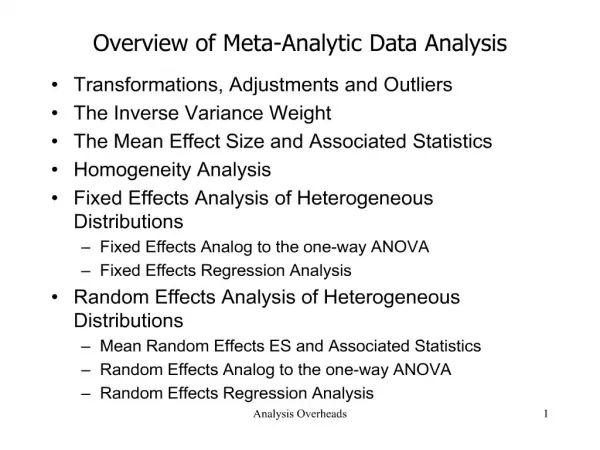
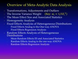
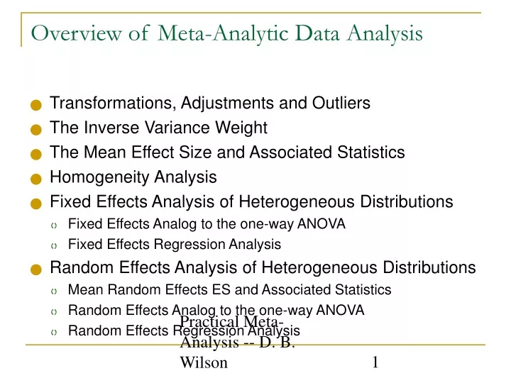
Practical Meta-Analysis -- D. B. Wilson Overview of Meta-Analytic Data Analysis • Transformations, Adjustments and Outliers • The Inverse Variance Weight • The Mean Effect Size and Associated Statistics • Homogeneity Analysis • Fixed Effects Analysis of Heterogeneous Distributions • Fixed Effects Analog to the one-way ANOVA • Fixed Effects Regression Analysis • Random Effects Analysis of Heterogeneous Distributions • Mean Random Effects ES and Associated Statistics • Random Effects Analog to the one-way ANOVA • Random Effects Regression Analysis
Practical Meta-Analysis -- D. B. Wilson Transformations • Some effect size types are not analyzed in their “raw” form. • Standardized Mean Difference Effect Size • Upward bias when sample sizes are small • Removed with the small sample size bias correction
Practical Meta-Analysis -- D. B. Wilson Transformations (continued) • Correlation has a problematic standard error formula. • Recall that the standard error is needed for the inverse variance weight. • Solution: Fisher’s Zr transformation. • Finally results can be converted back into “r” with the inverse Zr transformation (see Chapter 3).
Practical Meta-Analysis -- D. B. Wilson Transformations (continued) • Analyses performed on the Fisher’s Zr transformed correlations. • Finally results can be converted back into “r” with the inverse Zr transformation.
Practical Meta-Analysis -- D. B. Wilson Transformations (continued) • Odds-Ratio is asymmetric and has a complex standard error formula. • Negative relationships indicated by values between 0 and 1. • Positive relationships indicated by values between 1 and infinity. • Solution: Natural log of the Odds-Ratio. • Negative relationship < 0. • No relationship = 0. • Positive relationship > 0. • Finally results can be converted back into Odds-Ratios by the inverse natural log function.
Practical Meta-Analysis -- D. B. Wilson Transformations (continued) • Analyses performed on the natural log of the Odds- Ratio: • Finally results converted back via inverse natural log function:
Practical Meta-Analysis -- D. B. Wilson Adjustments • Hunter and Schmidt Artifact Adjustments • measurement unreliability (need reliability coefficient) • range restriction (need unrestricted standard deviation) • artificial dichotomization (correlation effect sizes only) • assumes an underlying distribution that is normal • Outliers • extreme effect sizes may have disproportionate influence on analysis • either remove them from the analysis or adjust them to a less extreme value • indicate what you have done in any written report
Practical Meta-Analysis -- D. B. Wilson Overview of Transformations, Adjustments,and Outliers • Standard transformations • sample sample size bias correction for the standardized mean difference effect size • Fisher’s Z to r transformation for correlation coefficients • Natural log transformation for odds-ratios • Hunter and Schmidt Adjustments • perform if interested in what would have occurred under “ideal” research conditions • Outliers • any extreme effect sizes have been appropriately handled
Practical Meta-Analysis -- D. B. Wilson Independent Set of Effect Sizes • Must be dealing with an independent set of effect sizes before proceeding with the analysis. • One ES per study OR • One ES per subsample within a study
Practical Meta-Analysis -- D. B. Wilson The Inverse Variance Weight • Studies generally vary in size. • An ES based on 100 subjects is assumed to be a more “precise” estimate of the population ES than is an ES based on 10 subjects. • Therefore, larger studies should carry more “weight” in our analyses than smaller studies. • Simple approach: weight each ES by its sample size. • Better approach: weight by the inverse variance.
Practical Meta-Analysis -- D. B. Wilson What is the Inverse Variance Weight? • The standard error (SE) is a direct index of ES precision. • SE is used to create confidence intervals. • The smaller the SE, the more precise the ES. • Hedges’ showed that the optimal weights for meta-analysis are:
Practical Meta-Analysis -- D. B. Wilson Inverse Variance Weight for theThree Common Effect Sizes • Standardized Mean Difference: • Zr transformed Correlation Coefficient:
Practical Meta-Analysis -- D. B. Wilson Inverse Variance Weight for theThree Major League Effect Sizes • Logged Odds-Ratio: Where a, b, c, and d are the cell frequencies of a 2 by 2 contingency table.
Practical Meta-Analysis -- D. B. Wilson Ready to Analyze • We have an independent set of effect sizes (ES) that have been transformed and/or adjusted, if needed. • For each effect size we have an inverse variance weight (w).
The Weighted Mean Effect Size • Start with the effect size (ES) and inverse variance weight (w) for 10 studies. Practical Meta-Analysis -- D. B. Wilson
The Weighted Mean Effect Size • Start with the effect size (ES) and inverse variance weight (w) for 10 studies. • Next, multiply w by ES. Practical Meta-Analysis -- D. B. Wilson
The Weighted Mean Effect Size • Start with the effect size (ES) and inverse variance weight (w) for 10 studies. • Next, multiply w by ES. • Repeat for all effect sizes. Practical Meta-Analysis -- D. B. Wilson
The Weighted Mean Effect Size • Start with the effect size (ES) and inverse variance weight (w) for 10 studies. • Next, multiply w by ES. • Repeat for all effect sizes. • Sum the columns, w and ES. • Divide the sum of (w*ES) by the sum of (w). Practical Meta-Analysis -- D. B. Wilson
The Standard Error of the Mean ES • The standard error of the mean is the square root of 1 divided by the sum of the weights. Practical Meta-Analysis -- D. B. Wilson
Practical Meta-Analysis -- D. B. Wilson Mean, Standard Error,Z-test and Confidence Intervals Mean ES SE of the Mean ES Z-test for the Mean ES 95% Confidence Interval
Practical Meta-Analysis -- D. B. Wilson Homogeneity Analysis • Homogeneity analysis tests whether the assumption that all of the effect sizes are estimating the same population mean is a reasonable assumption. • Assumption rarely reasonable • Single mean ES not a good descriptor of the distribution • There are real between study differences, that is, studies estimate different population mean effect sizes • Random effects model addresses this issue • You can also explore this excess variability with moderator analysis
Q - The Homogeneity Statistic • Calculate a new variable that is the ES squared multiplied by the weight. • Sum new variable. Practical Meta-Analysis -- D. B. Wilson
Practical Meta-Analysis -- D. B. Wilson Calculating Q We now have 3 sums: Q is can be calculated using these 3 sums:
Practical Meta-Analysis -- D. B. Wilson Interpreting Q • Q is distributed as a Chi-Square • df = number of ESs - 1 • Running example has 10 ESs, therefore, df = 9 • Critical Value for a Chi-Square with df = 9 and p = .05 is: • Since our Calculated Q (14.76) is less than 16.92, we fail to reject the null hypothesis of homogeneity. • Thus, the variability across effect sizes does not exceed what would be expected based on sampling error. 16.92
Practical Meta-Analysis -- D. B. Wilson Heterogeneous Distributions: What Now? • Analyze excess between study (ES) variability • categorical variables with the analog to the one-way ANOVA • continuous variables and/or multiple variables with weighted multiple regression
Analyzing Heterogeneous Distributions:The Analog to the ANOVA • Calculate the 3 sums for each subgroup of effect sizes. A grouping variable (e.g., random vs. nonrandom) Practical Meta-Analysis -- D. B. Wilson
Practical Meta-Analysis -- D. B. Wilson Analyzing Heterogeneous Distributions:The Analog to the ANOVA Calculate a separate Q for each group:
Practical Meta-Analysis -- D. B. Wilson Analyzing Heterogeneous Distributions:The Analog to the ANOVA The sum of the individual group Qs = Q within: Where k is the number of effect sizes and j is the number of groups. The difference between the Q total and the Q within is the Q between: Where j is the number of groups.
Practical Meta-Analysis -- D. B. Wilson Analyzing Heterogeneous Distributions:The Analog to the ANOVA All we did was partition the overall Q into two pieces, a within groups Q and a between groups Q. The grouping variable accounts for significant variability in effect sizes.
Practical Meta-Analysis -- D. B. Wilson Mean ES for each Group The mean ES, standard error and confidence intervals can be calculated for each group:
Practical Meta-Analysis -- D. B. Wilson Analyzing Heterogeneous Distributions:Multiple Regression Analysis • Analog to the ANOVA is restricted to a single categorical between studies variable. • What if you are interested in a continuous variable or multiple between study variables? • Weighted Multiple Regression Analysis • as always, it is weighted analysis • can use “canned” programs (e.g., SPSS, SAS) • parameter estimates are correct (R-squared, B weights, etc.) • F-tests, t-tests, and associated probabilities are incorrect • can use Wilson/Lipsey SPSS macros which give correct parameters and probability values
Practical Meta-Analysis -- D. B. Wilson Meta-Analytic Multiple Regression ResultsFrom the Wilson/Lipsey SPSS Macro(data set with 39 ESs) ***** Meta-Analytic Generalized OLS Regression ***** ------- Homogeneity Analysis ------- Q df p Model 104.9704 3.0000 .0000 Residual 424.6276 34.0000 .0000 ------- Regression Coefficients ------- B SE -95% CI +95% CI Z P Beta Constant -.7782 .0925 -.9595 -.5970 -8.4170 .0000 .0000 RANDOM .0786 .0215 .0364 .1207 3.6548 .0003 .1696 TXVAR1 .5065 .0753 .3590 .6541 6.7285 .0000 .2933 TXVAR2 .1641 .0231 .1188 .2094 7.1036 .0000 .3298 Partition of total Q into variance explained by the regression “model” and the variance left over (“residual” ). Interpretation is the same as will ordinal multiple regression analysis. If residual Q is significant, fit a mixed effects model.
Practical Meta-Analysis -- D. B. Wilson Review of WeightedMultiple Regression Analysis • Analysis is weighted. • Q for the model indicates if the regression model explains a significant portion of the variability across effect sizes. • Q for the residual indicates if the remaining variability across effect sizes is homogeneous. • If using a “canned” regression program, must correct the probability values (see manuscript for details).
Practical Meta-Analysis -- D. B. Wilson Random Effects Models • Don’t panic! • It sounds worse than it is. • Four reasons to use a random effects model • Total Q is significant and you assume that the excess variability across effect sizes derives from random differences across studies (sources you cannot identify or measure) • The Q within from an Analog to the ANOVA is significant • The Q residual from a Weighted Multiple Regression analysis is significant • It is consistent with your assumptions about the distribution of effects across studies
Practical Meta-Analysis -- D. B. Wilson The Logic of aRandom Effects Model • Fixed effects model assumes that all of the variability between effect sizes is due to sampling error • In other words, instability in an effect size is due simply to subject-level “noise” • Random effects model assumes that the variability between effect sizes is due to sampling error plus variability in the population of effects (unique differences in the set of true population effect sizes) • In other words, instability in an effect size is due to subject-level “noise” and true unmeasured differences across studies (that is, each study is estimating a slightly different population effect size)
Practical Meta-Analysis -- D. B. Wilson The Basic Procedure of aRandom Effects Model • Fixed effects model weights each study by the inverse of the sampling variance. • Random effects model weights each study by the inverse of the sampling variance plus a constant that represents the variability across the population effects. This is the random effects variance component.
Practical Meta-Analysis -- D. B. Wilson How To Estimate the RandomEffects Variance Component • The random effects variance component is based on Q. • The formula is:
Calculation of the RandomEffects Variance Component • Calculate a new variable that is the w squared. • Sum new variable. Practical Meta-Analysis -- D. B. Wilson
Practical Meta-Analysis -- D. B. Wilson Calculation of the RandomEffects Variance Component • The total Q for this data was 14.76 • k is the number of effect sizes (10) • The sum of w = 269.96 • The sum of w2 = 12,928.21
Practical Meta-Analysis -- D. B. Wilson Rerun Analysis with NewInverse Variance Weight • Add the random effects variance component to the variance associated with each ES. • Calculate a new weight. • Rerun analysis. • Congratulations! You have just performed a very complex statistical analysis. • Note: Macros do this for you. All you need to do is specify “model = mm” or “model = ml”
Practical Meta-Analysis -- D. B. Wilson Random Effects Variance Component for the Analog to the ANOVA and Regression Analysis • The Q between or Q residual replaces the Q total in the formula. • Denominator gets a little more complex and relies on matrix algebra. However, the logic is the same. • SPSS macros perform the calculation for you.
Practical Meta-Analysis -- D. B. Wilson SPSS Macro Output with Random EffectsVariance Component ***** Inverse Variance Weighted Regression ***** ***** Random Intercept, Fixed Slopes Model ***** ------- Descriptives ------- Mean ES R-Square k .1483 .2225 38.0000 ------- Homogeneity Analysis ------- Q df p Model 14.7731 3.0000 .0020 Residual 51.6274 34.0000 .0269 Total 66.4005 37.0000 .0021 ------- Regression Coefficients ------- B SE -95% CI +95% CI Z P Beta Constant -.6752 .2392 -1.1439 -.2065 -2.8233 .0048 .0000 RANDOM .0729 .0834 -.0905 .2363 .8746 .3818 .1107 TXVAR1 .3790 .1438 .0972 .6608 2.6364 .0084 .3264 TXVAR2 .1986 .0821 .0378 .3595 2.4204 .0155 .3091 ------- Method of Moments Random Effects Variance Component ------- v = .04715 Random effects variance component based on the residual Q.
Practical Meta-Analysis -- D. B. Wilson Comparison of Random Effect with Fixed Effect Results • The biggest difference you will notice is in the significance levels and confidence intervals. • Confidence intervals will get bigger. • Effects that were significant under a fixed effect model may no longer be significant. • Random effects models are therefore more conservative. • If sample size is highly related to effect size, then the mean effect size will differ between the two models
Practical Meta-Analysis -- D. B. Wilson Review of Meta-Analytic Data Analysis • Transformations, Adjustments and Outliers • The Inverse Variance Weight • The Mean Effect Size and Associated Statistics • Homogeneity Analysis • Fixed Effects Analysis of Heterogeneous Distributions • Fixed Effects Analog to the one-way ANOVA • Fixed Effects Regression Analysis • Random Effects Analysis of Heterogeneous Distributions • Mean Random Effects ES and Associated Statistics • Random Effects Analog to the one-way ANOVA • Random Effects Regression Analysis