Download
1 / 37
390 likes | 459 Views
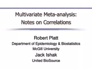
An overview of meta-analysis in Stata Part II: multivariate meta-analysis. Ian White MRC Biostatistics Unit, Cambridge Stata Users’ Group London, 10 th September 2010. Plan. Example 1: Berkey data Multivariate random-effects meta-analysis model Situations where it could be used

E N D
An overview of meta-analysis in StataPart II: multivariate meta-analysis Ian White MRC Biostatistics Unit, Cambridge Stata Users’ Group London, 10th September 2010
Plan • Example 1: Berkey data • Multivariate random-effects meta-analysis model • Situations where it could be used • Software: mvmeta • A problem: unknown within-study correlation • Example 2: fibrinogen • software: mvmeta_make • Multivariate vs. univariate
Example from Berkey et al (1998) • 5 trials comparing a surgical with a non-surgical procedure for treating periodontal disease • 2 outcomes: • “probing depth” (PD) • “attachment level” (AL) y1,y2 - treatment effects for PD, AL; s1,s2 - standard errors
Berkey data (1) • Could analyse the outcomes one by one Random effects weight Random effects weight Study ID Study ID 1 19.71 19.71 1 17.82 17.82 2 22.05 22.05 2 19.84 19.84 3 21.83 21.83 3 25.64 25.64 4 21.79 21.79 4 24.08 24.08 5 14.61 14.61 5 12.62 12.62 100.00 100.00 Overall 100.00 100.00 Overall I2 = 68.8%, p = 0.012 I2 = 96.4%, p = 0.000 -1 -.5 0 0 0 0 .5 1 Mean improvement in attachment level Mean improvement in probing depth
0 -.2 -.4 Mean improvement in attachment level -.6 -.8 0 .2 .4 .6 .8 Mean improvement in probing depth Berkey data (2) • Dots mark the point estimates for the 5 studies • Bubbles show 50% confidence regions • Note the positive within-study correlation (0.3-0.4 for all studies) • bubble.ado, available on my website 3 4 5 1 2
One or two stages? • I’m assuming a two-stage meta-analysis (as in the Berkey data): • 1st stage: compute results for each study • 2nd stage: use these results as “data” • makes a Normal approximation to the within-study log-likelihoods • One-stage meta-analysis is possible if we have individual participant data (IPD), but can be computationally horrible (Smith et al 2005) • we’ll use the two-stage method even with IPD
Bivariate meta-analysis: data • Data from ith study: • yi1, yi2 – estimates for 1st, 2nd outcomes • si1, si2– their standard errors • but we also need the correlationrWiof yi1and yi2 • It’s often most convenient to use matrix notation: estimate with within-study variance • NB yi1or yi2 can be missing.
Bivariate meta-analysis: the model • Data from ith study: • yi – vector of estimates • Si – variance-covariance matrix • Model is yi ~ N(m, Si+S) • Total variance = within + between variance: known to be estimated
Bivariate meta-analysis: 2 correlations • Within-study correlation rWi • one per study • should be known from 1st stage of meta-analysis • but often unknown: discussed later • Between-study correlation rB • overall parameter • to be estimated
Multivariate meta-analysis: the model • Data from ith study: • yi – vector of estimates (p-dimensional) • Si – variance-covariance matrix (pxp) • Model is again yi ~ N(m, Si+S) • Can also extend to meta-regression: e.g. yi ~ N(bxi, Si+S) • xiis a q–dimensional vector of explanatory variables • b is a pxq matrix containing the regression coefficients for each of the p outcomes • more generally, can allow different x’s for different outcomes
When could multivariate meta-analysis be used? (1) • Original applications: meta-analysis of randomised controlled trials (RCTs) • several outcomes of interest • some trials report more than one outcome • “data” are treatment effects on each outcome in each study (some may be missing) • data are correlated within studies because outcomes are correlated • also used in health economics for cost and effect (Pinto et al, 2005)
When could multivariate meta-analysis be used? (2) • Meta-analysis of diagnostic accuracy studies • “data” are sensitivity and specificity in each study • data are uncorrelated within studies because they refer to different subgroups • still likely to be correlated between studies • See Roger’s talk • sparse data often invalidates Normal approximation • best to use metandi
When could multivariate meta-analysis be used? (3) • Meta-analysis of RCTs comparing more than two treatments • “data” are treatment effects for each treatment compared to same control • data are correlated within studies because they use same control group • Similarly multiple treatments meta-analysis • my current area of research
When could multivariate meta-analysis be used? (4) • Meta-analysis of observational studies exploring shape of exposure-disease relationship • if exposure is categorised, “data” could be contrasts between categories • if fractional polynomial model is used, “data” would be coefficients of different model terms
Stata software for multivariate random-effects meta-analysis • Can almost use xtmixed • but you need to constrain the level 1 (co)variances • not possible in xtmixed • So I wrote mvmeta (White, 2009)
My program: mvmeta • Analyses a data set containing point estimates with their (within-study) variances and covariances • Utility mvmeta_make creates a data set in the correct format (demo later) • Fits random-effects model • uses ml to maximise the (restricted) likelihood using numerical derivatives • between-studies variance-covariance matrix is parameterised via its Cholesky decomposition • CIs are based on Normal distribution • also offers method of moments estimation (Jackson et al, 2009)
Data format for mvmeta: Berkey data y1, y2 treatment effects for PD, AL V11, V22 squared standard errors (si12, si22) V12 covariance (rWisi1si2)
Running mvmeta: Berkey data . mvmeta y V Note: using method reml Note: using variables y1 y2 Note: 5 observations on 2 variables [5 iterations] Number of obs = 5 Wald chi2(2) = 93.15 Log likelihood = 2.0823296 Prob > chi2 = 0.0000 ------------------------------------------------------------------------------ | Coef. Std. Err. z P>|z| [95% Conf. Interval] -------------+---------------------------------------------------------------- Overall_mean | y1 | .3534282 .061272 5.77 0.000 .2333372 .4735191 y2 | -.3392152 .08927 -3.80 0.000 -.5141811 -.1642493 ------------------------------------------------------------------------------ Estimated between-studies SDs and correlation matrix: SD y1 y2 y1 .1083191 1 .60879876 y2 .1806968 .60879876 1
Running mvmeta: method of moments . mvmeta y V, mm Note: using method mm (truncated) Note: using variables y1 y2 Note: 5 observations on 2 variables Multivariate meta-analysis Method = mm Number of dimensions = 2 Number of observations = 5 ------------------------------------------------------------------------------ | Coef. Std. Err. z P>|z| [95% Conf. Interval] -------------+---------------------------------------------------------------- y1 | .3478429 .0557943 6.23 0.000 .238488 .4571978 y2 | -.3404843 .1131496 -3.01 0.003 -.5622534 -.1187152 ------------------------------------------------------------------------------ Estimated between-studies SDs and correlation matrix: SD y1 y2 y1 .10102601 1 .74742532 y2 .23937024 .74742532 1
Running mvmeta: I2 • I2 measures the impact of heterogeneity (Higgins & Thompson, 2002) . mvmeta1 y V, i2 [output omitted] I-squared statistics: -------------------------------------------------- Variable I-squared [95% Conf. Interval] -------------------------------------------------- y1 72% -45% 94% y2 94% 76% 98% -------------------------------------------------- (computed from estimated between and typical within variances) • Requires updated mvmeta1
Running mvmeta: meta-regression . mvmeta1 y V publication_year, reml dof(n-2) Note: using method reml Note: using variables y1 y2 Note: 5 observations on 2 variables Variance-covariance matrix: unstructured [4 iterations] Multivariate meta-analysis Method = reml Number of dimensions = 2 Restricted log likelihood = -5.3778317 Number of observations = 5 Degrees of freedom = 3 ------------------------------------------------------------------------------ | Coef. Std. Err. z P>|z| [95% Conf. Interval] -------------+---------------------------------------------------------------- y1 | publicatio~r | .0048615 .02223470.22 0.841 -.0658992 .0756221 _cons | .3587569 .0740749 4.84 0.017 .1230175 .5944963 -------------+---------------------------------------------------------------- y2 | publicatio~r | -.0115367 .0303001-0.38 0.729 -.107965 .0848917 _cons | -.3357368 .0985988 -3.41 0.042 -.6495222 -.0219513 ------------------------------------------------------------------------------
mvmeta: programming • Basic parameters: Cholesky decomposition of the between-studies variance S • Eliminate fixed parameters from (restricted) likelihood • Maximise using ml, method d0 (can’t use lf for REML) • Likelihood now coded in Mata • Stata creates matrices yi , Sifor each study & sends them to Mata
Estimating the within-study correlation ρwi • Sometimes known to be 0 • e.g. in diagnostic test studies where sens and spec are estimated on different subgroups • Estimation usually requires IPD • even then, not always trivial: e.g. for 2 outcomes in RCTs, can fit seemingly unrelated regressions, or observe ρwi = correlation of the outcomes • Published literature never (?) reports ρwi • not the objective of the original study • difficult to estimate from summary data • What do we do in a published literature meta-analysis if ρwi values are missing?
Unknown ρwi: possible solutions • Ignore within-study correlation (set ρwi= 0) • not advisable (Riley, 2009) • Sensitivity analysis using a range of values • can be time-consuming & confusing • Use external evidence (e.g. IPD on one study) • Bayesian approach (Nam et al., 2004) • e.g. ρwi~U(0,1) • Some special cases where it can be done • % survival at multiple time-points • nested binary outcomes? • Use an alternative model that models the ‘overall’ correlation (Riley et al., 2008)
Standard model with overall rB and one rWi per study: Alternative bivariate model Alternative model with one ‘overall’ correlation r: mvmeta1: corr(riley) option
Example: Fibrinogen • Fibrinogen Studies Collaboration (2005) • assembled IPD from 31 observational studies • 154211 participants • to explore the association between fibrinogen levels (measured in blood) and coronary heart disease • We focus on exploring the shape of the association using grouped fibrinogen • Data (IPD): • Variable fg contains fibrinogen in 5 groups • Studies are identified by variable cohort • Time to CHD has been stset • In each cohort, I want to run the Cox modelxi: stcox age i.fg, strata(sex tr)
1st stage of meta-analysis: mvmeta_make • Getting IPD into the right format can be the hardest bit • I wrote mvmeta_make to do this • It assumes the 1st stage of meta-analysis involves fitting a regression model
Fibrinogen data: using mvmeta_make • Stata command within each study: • xi: stcox age i.fg, strata(sex tr) • Create meta-analysis data set: • xi: mvmeta_make stcox age i.fg, strata(sex tr) by(cohort) usevars(i.fg) name(b V) saving(FSC2) • Creates file FSC2.dta containing • coefficients: b_Ifg_2, b_Ifg_3, b_Ifg_4, b_Ifg_5 • variances and covariances: V_Ifg_2_Ifg_2, V_Ifg_2_Ifg_3 etc. • We then run mvmeta b V on file FSC2.dta.
A problem: perfect prediction . tab fg allchd if cohort=="KORA_S3" Fibrinogen | Any CHD event? groups | 0 1 | Total -----------+----------------------+---------- 1 | 546 0 | 546 2 | 697 3 | 700 3 | 715 2 | 717 4 | 677 4 | 681 5 | 482 8 | 490 -----------+----------------------+---------- Total | 3,117 17 | 3,134 • No events in the reference category • Fit Cox model: HR for 2 vs 1 is 21.36 (se 0.91) – wrong
mvmeta_make: handling perfect prediction • Recall: • no events in fg=1 (reference) group • stcox’s “fix” can yield large hazard ratios with small standard errors – and disaster for mvmeta! • mvmeta_make implements a different “fix” in any study with perfect prediction: • add a few observations, with very small weight, that “break” the perfect prediction • all contrasts with fg=1 are large with large s.e. • all other contrasts (e.g. fg=3 vs. fg=2) are correct • Works fine for likelihood-based procedures (REML, ML, fixed-effect model) but not for method of moments
Study with no events in fg=1 group: “perfect prediction” FSC: partial results of mvmeta_make . l c b* V_Ifg_2_Ifg_2 V_Ifg_3_Ifg_3 , clean noo cohort b_Ifg_2 b_Ifg_3 b_Ifg_4 b_Ifg_5 V_Ifg_~2 ~3_Ifg_3 ARIC 0.252 0.532 0.946 1.401 0.036 0.033 BRUN -0.184 -0.032 0.119 0.567 0.348 0.344 CAER 0.001 -0.529 -0.339 0.416 0.375 0.323 CHS 0.066 0.184 0.407 0.645 0.058 0.053 COPEN 0.078 0.406 0.544 1.088 0.101 0.083 EAS -0.113 0.456 0.456 0.875 0.065 0.054 FINRISKI -2.149 -0.264 -0.494 0.169 1.336 0.421 FRAM -0.039 0.170 0.420 1.053 0.042 0.038 GOTO 0.443 0.595 0.922 0.797 0.202 0.175 GOTO33 0.356 1.312 0.628 2.133 1.500 1.170 GRIPS 1.297 1.052 1.421 1.752 0.559 0.542 HONOL 0.323 0.545 0.681 0.540 0.132 0.122 KIHD -0.042 0.509 0.560 0.998 0.088 0.072 KORA_S2 -2.667 -2.524 -2.010 -1.767 1.337 0.584 KORA_S3 5.946 5.420 6.088 7.057 189.088 189.271 MALMO 0.123 0.371 0.506 0.936 0.071 0.058 ...
FSC: results of mvmeta . mvmeta b V Number of obs = 31 Wald chi2(4) = 142.62 Log likelihood = -79.129029 Prob > chi2 = 0.0000 -------------------------------------------------------------------- | Coef. Std. Err. z P>|z| [95% Conf. Int.] -------------+------------------------------------------------------ Overall_mean | b_Ifg_2 | .1646353 .0787025 2.09 0.036 .0103813 .3188894 b_Ifg_3 | .3905063 .088062 4.43 0.000 .2179080 .5631047 b_Ifg_4 | .5612908 .0904966 6.20 0.000 .3839206 .7386609 b_Ifg_5 | .8998468 .0932989 9.64 0.000 .7169843 1.082709 -------------------------------------------------------------------- Estimated between-studies variance matrix Sigma: b_Ifg_2 b_Ifg_3 b_Ifg_4 b_Ifg_5 b_Ifg_2 .04945818 b_Ifg_3 .06355581 .0836853 b_Ifg_4 .06689067 .08920553 .09570788 b_Ifg_5 .0506146 .07530983 .08501967 .1041611
FSC: graphical results Other choices of reference category give the same results.
Example 2: borrowing strength • y2>0 ⇒ y1 missing • y2<0 ⇒ y1 observed • Pooling the observed y1 can’t be a good way to estimate m1 • Bivariate model helps: • assumes a linear regression of m1 on m2 • assumes data are missing at random • Bivariate model can avoid bias & increase precision (“Borrowing strength”)
Multivariate vs. univariate meta-analysis • Advantages: • “borrowing strength” • avoiding bias from selective outcome reporting • Joint confidence / prediction intervals • Functions of estimates • Longitudinal data • Coherence • Disadvantages: • more computationally complex • boundary solutions for rB • unknown within-study correlations • more assumptions
Getting mvmeta • mvmeta is in the SJ • Current update mvmeta1 is available on my website (includes meta-regression, I2, structured S, speed & other improvements) • net from http://www.mrc‑bsu.cam.ac.uk/IW_Stata • bubble is also available
References Berkey CS et al. Meta-analysis of multiple outcomes by regression with random effects. Statistics in Medicine 1998;17:2537–2550. Fibrinogen Studies Collaboration. Plasma fibrinogen and the risk of major cardiovascular diseases and non-vascular mortality. JAMA 2005; 294: 1799–1809. Higgins J, Thompson S. Quantifying heterogeneity in a meta-analysis. Statistics in Medicine 2002;21:1539–58. Jackson D, White I, Thompson S. Extending DerSimonian and Laird’s methodology to perform multivariate random effects meta-analyses. Statistics in Medicine 2009;28:1218-1237. Kenward MG, Roger JH. Small sample inference for fixed effects from restricted maximum likelihood. Biometrics 1997; 53: 983–997. Nam IS, Mengersen K, Garthwaite P. Multivariate meta-analysis. Statistics in Medicine 2003; 22: 2309–2333. Pinto E, Willan A, O’Brien B. Cost-effectiveness analysis for multinational clinical trials. Statistics in Medicine 2005;24:1965–82. Riley RD. Multivariate meta-analysis: the effect of ignoring within-study correlation. JRSSA 2009;172:789-811. Riley RD, Thompson JR, Abrams KR. An alternative model for bivariate random-effects meta-analysis when the within-study correlations are unknown. Biostatistics 2008; 9: 172-186 Smith CT, Williamson PR, Marson AG. Investigating heterogeneity in an individual patient data meta-analysis of time to event outcomes. Statistics In Medicine 2005;24:1307–1319. White IR. Multivariate random-effects meta-analysis. Stata Journal 2009;9:40–56.