Download
1 / 40
400 likes | 402 Views
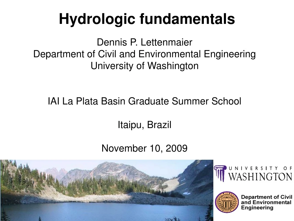
Hydrologic fundamentals. Dennis P. Lettenmaier Department of Civil and Environmental Engineering University of Washington IAI La Plata Basin Graduate Summer School Itaipu, Brazil November 10, 2009. Outline of this talk. Runoff generation processes

E N D
Hydrologic fundamentals Dennis P. Lettenmaier Department of Civil and Environmental Engineering University of Washington IAI La Plata Basin Graduate Summer School Itaipu, Brazil November 10, 2009
Outline of this talk Runoff generation processes The role of vegetation and the energy balance Spatially distributed vs spatially lumped hydrological models Channel routing and streamflow prediction
Darcy’s Equation (fundamental equation of motion in subsurface, applies to both saturated and unsaturated zones): whereq = flow per unit cross-sectional area (units L/T) K = hydraulic conductivity (L/T) Definitions: = volume of water/total volume η = porosity (volume of voids/total volume = suction head (height to which moisture is drawn above free surface
let = diffusivity From continuity Combining, (Richard’s equation)
Applies at point scale, “well behaved” porous medium K is highly nonlinear spatially varying function of suction head, moisture K varies over orders of magnitude due to variations in soil properties at meter scales (much less than typical scale of application) Direct estimation of K difficult even at small scale (and scale complications in interpretation of measurements) Methods of estimating K from e.g. mapable soil properties are highly approximate, and subject to scale complications Complications in the application of Richards Equation
1) Infiltration excess – precipitation rate exceeds local (vertical) hydraulic conductivity -- typically occurs over low permeability surfaces, e.g., arid areas with soil crusting, frozen soils 2) Saturation excess – “fast” runoff response over saturated areas, which are dynamic during storms and seasonally (defined by interception of the water table with the surface) Runoff generation mechanisms
Runoff generation mechanisms on a hillslope (source: Dunne and Leopold)
Seasonal contraction of saturated area at Sleepers River, VT following snowmelt (source: Dunne and Leopold)
Expansion of saturated area during a storm (source: Dunne and Leopold)
Seasonal contraction of pre-storm saturated areas, Sleepers River VT (source: Dunne and Leopold)
Classical hydrological models typically prescribe a) precipitation b) PET -- AET is computed as a fraction of PET, where the fraction depends on soil moisture storage (variation of Budyko curve, where ET/PET = f(W/Wc), where W is soil moisture, and Wc is soil moisture capacity) AET is then estimated either from time-varying meteorological forcings or (more often) is seasonally fixed. Model parameters are calibrated so as to reproduce observed streamflow given precipitation These methods have a critical limitation if either climate or land cover changes, but can work well for applied purposes (e.g. flood forecasting) otherwise
If a land surface model is to be used in a coupled land-atmosphere context, it must close both the energy and water balances This motivation lead to the class of SVATS (Soil-Vegetation-Atmosphere Transfer Schemes) in the 1980s. These models explicitly represent the role of biophysical processes as they control evapotranspiration and photosynthesis These models had as their primary motivation accurate partitioning of Rnet into latent, sensible, and ground heat flux, while utilizing available information about land cover. These models mostly did not represent runoff generation processes well however – they tended to place more emphasis on representation of “vertical” processes controlling evaporative and energy fluxes, and less (or none) on spatial heterogeneity, which is the dominant factor that controls runoff production In fact, runoff and evap are linked (since they have to add to precipitation in the long-term mean), so it doesn’t make sense to emphasize one relative to the other. SVATS-based approaches
The role of vegetation on surface moisture and energy fluxes
Smaller Sub-watersheds More realistic Processes • Streamflow (at predetermined points) • Predictive skill limited to calibration conditions Streamflow Snow Runoff Soil Moisture, etc at all points and areas in the basin Predictive Skill Outside Calibration Conditions. 3. Spatially distributed vs spatially lumped hydrologic models Lumped Conceptual Fully Distributed Physically-based Suitable for flood forecasting and a wide range of water resource related issues Suitable for flood forecasting
Traditional “bottom up” hydrologic modeling approach (subbasin by subbasin)
Unit Hydrograph Theory • Concept dates to Sherman (1932) • The concept • Given two evenly distributed rainfall events over an entire watershed,l The response hydrographs of the watershed are assumed to have similar characteristics • The only difference will be in the magnitude of the flows • Mathematically the unit hydrograph is a convolution integral, where the UH weights represent the effects of a unit “pulse” of rainfall on streamflow at the basin outlet: • In practice, a major issue is determining the role of antecedent (soil moisture) conditions • Can be adapted so that the inputs are runoff, which is assumed (in the model world) to be a distributed quantity that is input at the grid cell level to the channel system (hence avoids the antecedent condition issue
Unit Hydrograph Theory Visual courtesy Michael Horst
Example • Given the following rainfall distribution • The watershed will respond as follows Visual courtesy Michael Horst
Example Visual courtesy Michael Horst
Example Visual courtesy Michael Horst
Other routing methods • Unit hydrograph has no physical basis, it is merely a convenient approximation to reality • Alternative routing methods are based, to varying degrees on approximations of the equations of fluid flow in open channels • While these methods can be more accurate, they generally are much more data intensive (e.g., require channel cross-sections, slope, and roughness), and computationally intensive • However, they may be warranted when the prediction interval of interest is not much longer than the basin response time (e.g. time of concentration).