Download
1 / 49
490 likes | 491 Views
This conference covers the introduction to gravitational wave astronomy, various detectors, data analysis methods, and future detector advancements. It includes topics such as compact binary inspirals, bursts from supernovae/GRBs, cosmological signals, and all-sky searches for continuous waves.

E N D
Gravitational WaveAstronomy IIIMichael LandryLIGO Hanford ObservatoryCalifornia Institute of Technologyon behalf of the LIGO Scientific Collaborationhttp://www.ligo.orgCERN Oct 16-18, 2006 Supernova remnant Cas A Credit: NASA/CXC/GSFC/U. Hwang et al.
Overview • Day 1 : Introduction. Sources. Detectors. • An introduction to gravitational wave astronomy • What are gravitational waves • Sources • Brief survey of detectors: bars, ground-based interferometers (each with one or two highlights), LISA • Day 2 : Ground-based interferometry • Interferometric detectors • LIGO, GEO, Virgo • Some topics in commissioning: the path to design sensitivity • Science mode running with LIGO, GEO and TAMA • Day 3 : Data analysis. Future detectors. • Search methods • Analyses from science runs for inspiral, burst, stochastic and continuous wave sources • Advanced LIGO, Advanced Virgo
What makes gravitational waves? • Compact binary inspiral: “chirps” • NS-NS waveforms are well described • BH-BH need better waveforms • Supernovae / GRBs: “bursts” • burst signals in coincidence with signals in electromagnetic radiation / neutrinos • all-sky untriggered searches too • Cosmological Signal: “stochastic background” • Pulsars in our galaxy:“continuous waves” • search for observed neutron stars • all-sky search (computing challenge)
Both IGEC2 bars and LSC results Signal duration and template
G.F. Prodi, INFN IGEC2 collab. First results by IGEC2 6 month of data of AURIGA-EXPLORER-NAUTILUS May 20 - Nov 15, 2005 IGEC2 was the only gw observatory in operation search for transient gw signals to identify single candidateswith high confidence : triple coincidences false alarm rate of 1 per century wider target signals than IGEC1 no candidates found
G.F. Prodi, INFN IGEC2 collab. IGEC2 search for bursts • perform only ONE composite search made by • the OR among the following data selections: • SNR > 4.95 for AU, EX and NA 0.396 false alarm /century targets signals peaked on EX-NA sweet spots • SNR > 7.00 for AU, SNR>4.25 for EX and NA 0.572 false alarm /century targets signals barely detectable by EX and NA • common absolute thresholds IGEC1-style: thresholds 1.3, 1.4, 1.5, ..., 3.0 x 10⁻²¹/Hz 0.134 false alarm /century targets -like signals 130 days of net simultaneous observation time by the three INFN resonant bar detectors
G.F. Prodi, INFN IGEC2 collab. IGEC2 Results • At last, we “opened the box” on Sept. 25 after exchanging the secret time shifts …no candidates were found.…the usual upper limit… • Comparison with the upper limits given by the IGEC 1997-2000 observations is possible using a subset of the current analysis: the IGEC1-style search targeting -like signals IGEC2 upper limit Burst Rate [year-1] 95% coverage Burst amplitude [Hz-1]
S2 untriggered burst search • bursts less than 1s, in band 100-1100Hz • 9.98d of data analyzed • Event triggers generated on triple-coincidence data, followed up by “r-statistic” waveform consistency test • Background set by similar analysis with time-shifted data • Set limit on rate of detectable gravitational wave bursts • Test efficiency of pipeline to detect particular waveforms: both ad hoc (gaussian, sine-gaussian) and astrophysically-motivated waveforms (core-collapse and binary black hole) applied • Set rate vs strength exclusion regions for these waveforms H1= LHO 4k H2= LHO 2kL1= LLO 4k Notation! :
Bursts: excess power detection • Now consider later runs, S3-S5 • Look for transient increase in power in some time-frequency region: • Minimal assumptions about signal • Duration: 1 to 100 ms • Characteristic time scale for stellar mass objects • Frequency: 60 to 2,000 Hz • Determined by detector's sensitivity • Many different implementations • Fourier modes, wavelets, sine-Gaussians • Multiple time/frequency resolutions • Provide redundancy and robustness Simulated binary inspiral signal in S5 data
Consistency Checks • Require time and frequency coincidence in three LIGO detectors. • Follow up coincidences with: • Amplitude consistency between co-located H1-H2 detectors • Cross correlation of data from pairs of detectors • Check environmental and auxiliary channels for: • Earthquakes, airplanes, trains, instrumental misbehaviour, ... • Remove times of poor data quality • Veto events associated to known noise sources • Compare remaining events with background estimated by repeating analysis with large time shifts of detector data.
Upper Limits • No GW bursts detected through S4 • set limit on rate vs signal strength. S1 Excluded 90% CL S2 Lower rate limits from longer observation times Rate Limit (events/day) S4 projected S5 projected Lower amplitude limits from lower detector noise
Inspiral and Merger of Compact Binaries • Binary Neutron Star Rates • Theoretical estimates give upper bound of 1/3yr for LIGO S5(Kalogera et. al, Ap J Lett 601, L179 (2004)) • n.b. Rates predicted for initial LIGO, based on identification of short GRBs as binary inspirals (astro-ph/0511254), higher than typical population synthesis modelling • Binary Black Hole Rates • Theoretical estimates give upper bound of 1/yr for LIGO S5 Best candidate for short GRBs: binary inspirals, NS-NS, BH-NS N. Gehrels et al., Nature 437, 851 (2005), and R. Narayan et al., Ap. J. Lett. 395 L83 (1992)
Target Sources • Use templated search • Require waveform consistency • Use detection templates for higher masses • Require time and mass coincidence between 2 or more detectors BBH: S2 – S5 Ringdown: S4 – S5 Coincidence with burst search 10 3 BNS S1 – S5 NS/BH spin important S3 – S5 Component Mass, M⊙ 1 PBH S2 – S5 0.1 0.1 1 3 10 Component Mass, M⊙
Binary Neutron Stars • S3 search complete • Under internal review • 0.09 yr of data • ~3 Milky-Way like galaxies for 1.4 – 1.4 M⊙ • S4 search complete • Under internal review • 0.05 yr of data • ~24 Milky-Way like galaxies for 1.4 – 1.4 M⊙ S2 Observational Result Phys. Rev. D. 72, 082001 (2005) Rate < 47 per year per Milky-Way-like galaxy; 0.04 yr data, 1.27 Milky-Ways cumulative number of events signal-to-noise ratio squared
S5 Binary Neutron Stars • First three months of S5 data have been analyzed • Horizon distance • Distance to 1.4-1.4 M⊙ optimally oriented & located binary at SNR 8 S2 Horizon Distance 1.5 Mpc H1: 25 Mpc L1: 21 Mpc H2: 10 Mpc Virgo Cluster
S5 Binary Black Holes • Horizon distance vs mass for BBH binary neutron star horizon distance Average over run 130Mpc 1 sigma variation Image: R. Powell binary black hole horizon distance Peak at total mass ~ 25M⊙
Search for stochastic gravitational waves • Cosmological relic, or, summation of noise sources from astrophysical epoch • Cross correlate detectors: uncorrelated noise integrates away while the signal to noise integrates up as the square root of time • Make use of optimal filter, which includes overlap reduction function • Searches include • LHO-LLO • H1-H2 • LLO-Allegro • WGW is the gravitational wave energy density per logarithmic frequency interval, divided by rc, the energy density required to close the universe
New S4 result (astro-ph/0608606): Bayesian 90% U.L. submitted to Ap. J. S4 stochastic background results Fake signal injected into LHO, LLO 4km instruments, then recovered
Search for continuous waves A B • Searches for g.w. : • Known pulsars • S4 all-sky (incoherent) • S3 all-sky (coherent) Mountain on neutron star Analysis goal for S5: hierarchical search Precessing neutron star Credits: A. image by Jolien Creighton; LIGO Lab Document G030163-03-Z. B. image by M. Kramer; Press Release PR0003, University of Manchester - Jodrell Bank Observatory, 2 August 2000. C. image by Dana Berry/NASA; NASA News Release posted July 2, 2003 on Spaceflight Now. D. image from a simulation by Chad Hanna and Benjamin Owen; B. J. Owen's research page, Penn State University. C Accreting neutron star D Oscillating neutron star LIGO-G060177-00-W
early S5 data Analyses for continuous gravitational waves I • S5 Time domain analysis • Targeted search of known objects: 73 pulsars with rotational frequencies > 25 Hz at known locations with phase inferred from radio data (knowledge of some parameters simplifies analysis) from the Jodrell Bank Pulsar Group (JBPG) and/or ATNF catalogue • Limit this search to gravitational waves from a neutron star (with asymmetry about its rotational axis) emitted at twice its rotational frequency, 2*frot • Signal would be frequency modulated by relative motion of detector and source, plus amplitude modulated by the motion of the antenna pattern of the detector • Analyzed from 4 Nov - 31 Dec 2005 using data from the three LIGO observatories Hanford 4k and 2k (H1, H2) and Livingston 4k (L1) • Upper limits defined in terms of Bayesian posterior probability distributions for the pulsar parameters • Validation by hardware injection of fake pulsars • Results
CW source model • F+ and Fx : strain antenna patterns of the detector to plus and cross polarization, bounded between -1 and 1 • Here, signal parameters are: • h0 – amplitude of the gravitational wave signal • y – polarization angle of signal • i – inclination angle of source with respect to line of sight • f0 – initial phase of pulsar; F(t=0), and F(t)= f(t) + f0 The expected signal has the form: Heterodyne, i.e. multiply by: so that the expected demodulated signal is then: Here, a = a(h0, y, i, f0), a vector of the signal parameters.
Aside: Injection of fake pulsars during S2 Parameters of P1: Two simulated pulsars, P1 and P2, were injected in the LIGO interferometers for a period of ~ 12 hours during S2 P1: Constant Intrinsic Frequency Sky position: 0.3766960246 latitude (radians) 5.1471621319 longitude (radians) Signal parameters are defined at SSB GPS time 733967667.026112310 which corresponds to a wavefront passing: LHO at GPS time 733967713.000000000 LLO at GPS time 733967713.007730720 In the SSB the signal is defined by f = 1279.123456789012 Hz fdot = 0 phi = 0 psi = 0 iota = p/2 h0 = 2.0 x 10⁻²¹ phase j0 recovered amplitude h0 injected amplitude h0 y cos i
Equatorial ellipticity • Results on h0 can be interpreted as upper limit on equatorial ellipticity • Ellipticity scales with the difference in radii along x and y axes • Distance r to pulsar is known, Izz is assumed to be typical, 1045 g cm2
S5 Results, 95% upper limits • Lowest h0 upper limit: • PSR J1603-7202 (fgw = 134.8 Hz, r = 1.6kpc) h0 = 1.6x10⁻²⁵ • Lowest ellipticity upper limit: • PSR J2124-3358 (fgw = 405.6Hz, r = 0.25kpc)e = 4.0x10⁻⁷ All values assume I = 1038 kgm2 and no error on distance PRELIMINARY
h0 Results • Closest to spin-down upper limit • Crab pulsar ~ 2.1 times greater than spin-down (fgw = 59.6 Hz, dist = 2.0 kpc) • h0 = 3.0x10⁻²⁴, e = 1.6x10⁻³ • Assumes I = 1038 kgm2 • Our upper limits are generally well above those permitted by spin-down constraints and neutron star equations-of-state • Our most stringent ellipticities (4.0x10⁻⁷) are starting to reach into the range of neutron star structures for some neutron-proton-electron models (B. Owen, PRL, 2005). Crab pulsar h0 Frequency (Hz) PRELIMINARY
Frequency Time Time Analyses for continuous gravitational waves II • “Stack Slide Method”: break up data into segments; FFT each, producing Short (30 min) Fourier Transforms (SFTs) = coherent step. • StackSlide: stack SFTs, track frequency, slide to line up & add the power weighted by noise inverse = incoherent step. • Other semi-coherent methods: • Hough Transform: Phys. Rev. D72 (2005) 102004; gr-qc/0508065. • PowerFlux • Fully coherent methods: • Frequency domain match filtering/maximum likelihood estimation Track Doppler shift and df/dt
PRELIMINARY Analysis of Hardware Injections Fake gravitational-wave signals corresponding to rotating neutron stars with varying degrees of asymmetry were injected for parts of the S4 run by actuating on one end mirror. Sky maps for the search for an injected signal with h0 ~ 7.5e-24 are below. Black stars show the fake signal’s sky position. DEC (degrees) DEC (degrees) RA (hours) RA (hours) LIGO-G060177-00-W
S4 StackSlide “Loudest Events” 50-225 Hz PRELIMINARY • Searched 450 freq. per .25 Hz band, 51 values of df/dt, between 0 & -1e-8 Hz/s, up to 82,120 sky positions (up to 2e9 templates). The expected loudest StackSlide Power was ~ 1.22 (SNR ~ 7) • Veto bands affected by harmonics of 60 Hz. • Simple cut: if SNR > 7 in only one IFO veto; if in both IFOs, veto if abs(fH1-fL1) > 1.1e-4*f0 StackSlide Power StackSlide Power Frequency (Hz) LIGO-Gxxxxxx-00-W
S4 StackSlide “Loudest Events” 50-225 Hz PRELIMINARY • Searched 450 freq. per .25 Hz band, 51 values of df/dt, between 0 & -1e-8 Hz/s, up to 82,120 sky positions (up to 2e9 templates). The expected loudest StackSlide Power was ~ 1.22 (SNR ~ 7) • Veto bands affected by harmonics of 60 Hz. • Simple cut: if SNR > 7 in only one IFO veto; if in both IFOs, veto if abs(fH1-fL1) > 1.1e-4*f0 FakePulsar3=> FakePulsar8=> StackSlide Power <=Follow-up Indicates Instrument Line FakePulsar8=> StackSlide Power FakePulsar3=> <=Follow-up Indicates Instrument Line Frequency (Hz) LIGO-Gxxxxxx-00-W
S4 StackSlide h0 95% Confidence All Sky Upper Limits 50-225 Hz PRELIMINARY Best: 4.4e-24 For 139.5-139.75 Hz Band S5: ~ 2x better sensitivity, 12x or more data This incoherent method (and other examples, Hough and Powerflux techniques) is one piece of hierarchical pipeline h0 Upper Limit Best: 5.4e-24 For 140.75-141.0 Hz Band h0 Upper Limit LIGO-Gxxxxxx-00-W Frequency (Hz)
Analyses for continuous gravitational waves III • All-sky search is computationally intensive, e.g. • searching 1 year of data, you have 3 billion frequencies in a 1000Hz band • For each frequency we need to search 100 million million independent sky positions • pulsars spin down, so you have to consider approximately one billion times more templates • Number of templates for each frequency: ~1023 • S3 Frequency-domain (“F-statistic”) all-sky search • The F-Statistic uses a matched filter technique, minimizing chisquare (maximizing likelihood) when comparing a template to the data • ~1015 templates search over frequency (50Hz-1500Hz) and sky position • For S3 we are using the 600 most sensitive hours of data • We are combining the results of multiple stages of the search incoherently using a coincidence scheme
What would a pulsar look like? • Post-processing step: find points on the sky and in frequency that exceeded threshold in many of the sixty ten-hour segments • Software-injected fake pulsar signal is recovered below Simulated (software) pulsar signal in S3 data
Final S3 analysis results • Data: 60 10-hour stretches of the best H1 data • Post-processing step on centralized server: find points in sky and frequency that exceed threshold in many of the sixty ten-hour segments analyzed • 50-1500 Hz band shows no evidence of strong pulsar signals in sensitive part of the sky, apart from the hardware and software injections. There is nothing “in our backyard”. • Outliers are consistent with instrumental lines. All significant artifacts away from r.n=0 are ruled out by follow-up studies. WITH INJECTIONS WITHOUT INJECTIONS
Einstein@home • Like SETI@home, but for LIGO/GEO data • American Physical Society (APS) publicized as part of World Year of Physics (WYP) 2005 activities • Use infrastructure/help from SETI@home developers for the distributed computing parts (BOINC) • Goal: pulsar searches using ~1 million clients. Support for Windows, Mac OSX, Linux clients • From our own clusters we can get ~ thousands of CPUs. From Einstein@home hope to get order(s) of magnitude more at low cost • Great outreach and science education tool • Currently : ~110,000 active users corresponding to about 42Tflops, about 250 new users/day http://einstein.phys.uwm.edu/
-18 10 -19 10 h (Hz-1/2) Pulsars hmax – 1 yr integration LIGO -20 10 Virgo -21 10 Resonant antennas GEO BH-BH Merger Oscillations -22 10 @ 100 Mpc Core Collapse QNM from BH Collisions, @ 10 Mpc QNM from BH Collisions, 100 - 10 Msun, 150 Mpc 1000 - 100 Msun, z=1 -23 10 BH-BH Inspiral, 100 Mpc NS-NS Merger Oscillations @ 100 Mpc BH-BH Inspiral, z = 0.4 -24 10 -6 e NS, =10 , 10 kpc 4 1 10 100 1000 10 NS-NS Inspiral, 300 Mpc P. Rapagnani Elba, 2006 Hz First Generation Detectors
Seismic Thermal Shot P. Rapagnani Elba, 2006 After 2007: Expanding the Accessible Universe: Where and how can we reduce the detector noise?
Advanced LIGO • Advanced LIGO is the LIGO Lab proposal for the next generation instrument to be installed at the LIGO Observatory Upgrade all 3 Interferometers and convert Hanford 2K to 4K Interferometer • Factor of 10 better amplitude sensitivity • Factor of 4 lower frequency bound • Potential for tunable, narrow band searches • Change transmission of recycling mirrors by changing mirrors or using tunable transmission mirror
Advanced LIGO LIGO detectors: future • Neutron Star Binaries: Initial LIGO: ~10-20 Mpc Advanced LIGO: ~200-350 Mpc Most likely rate: 1 every 2 days ! • Black hole Binaries: Up to 10 Mo, at ~ 100 Mpc up to 50 Mo, in most of the observable Universe! x10 better amplitude sensitivity x1000rate=(reach)3 1 year of Initial LIGO < 1 day of Advanced LIGO ! Planned NSF Funding in FY’08 budget.
INITIAL LIGO LAYOUT Test Masses M Arms of length L Cavity finesse F Michelson for sensing strain GW signal Fabry-Perot arms to increase interaction time Laser Power recycling mirror to increase circulating power Advanced LIGO Detector Improvements Retain infrastructure, vacuum chambers, and Initial LIGOlayout of power recycled interferometer • Replace passive seismic isolation with multi-staged system with inertial sensing and feedback control • Increase number of passive suspension isolation steps and use lower noise activation techniques • Use lower mechanical-loss materials and construction in suspensions, optical substrates and coatings to reduce thermal noise • Increase laser power ~20x and reduce optical losses to improve shot noise limits and signal strength • Add GW signal recycling at output to increase sensitivity and allow narrow band frequency tuning.
Full-Scale Seismic Prototypes & Early Implementation External pre-isolator installed and operating at Livingston • Performance meets initial LIGO and exceeds Advanced LIGO requirements Technology Demonstrator at Stanford in characterization • 1000x Isolation at GW frequencies demonstrated • 1-10 Hz performance testing in progress Planned future testing of full scale, integrated seismic isolation and suspensions at MIT’s test facility.
Thermal Noise Suppression • Minimise thermal noise from pendulum modes and their electronic controls • Thermally induced motion of the test masses sets the sensitivity limit in the range ~10 — 100 Hz • Required noise level at each of the main optics is 10–19 m/Hz at 10 Hz, falling off at higher frequencies • Choose quadruple pendulum suspensions for the main optics and triplependulum suspensions for less critical optics • Create quasi-monolithic pendulums using fused silica ribbons to suspend 40 kg test mass Silica fibres Test mass with mirror coating Silicate bonds
output NPRO EOM f f QR FI BP FI modematching YAG / Nd:YAG 3x2x6 optics f QR f BP YAG / Nd:YAG / YAG f 2f f HR@1064 3x 7x40x7 HT@808 20 W Master High Power Slave Shot Noise Limits • Increase laser power to lower shot noise • Require TEM00, stability in frequency and intensity • Significant motion due to photon pressure – quantum limited • ~180 W input power is practical limit • Increased laser power (~0.8MW in FP cavities) leads to increased requirements on many components • Photo-diodes, optical absorption, thermal lensing compensation, modulators and faraday isolators, etc. • Full injection locked master-slave system running, 200 W, linear polarization, single frequency, many hours of continuous operation
Projected Adv LIGO Detector Performance • Newtonian background,estimate for LIGO sites • Seismic ‘cutoff’ at 10 Hz • Suspension thermal noise • Test mass thermal noise • Unified quantum noise dominates at most frequencies for fullpower, broadband tuning Advanced LIGO's Fabry-Perot Michelson Interferometer is flexible – can tailor to what we learn before and after we bring it on line, to the limits of this topology and fundamental noise limits. 10-21 Initial LIGO 10-22 Strain Advanced LIGO 10-23 10-24 10 Hz 100 Hz 1 kHz
P. Rapagnani Elba, 2006 Advanced VIRGO 2006-2007 • Working groups activity • Signal Recycling • High Power • New optics and optical configuration • Technical design 2008-2009 • Engineering activities for Advanced Virgo > 2010 • Advanced Virgo upgrades
h (Hz-1/2) P. Rapagnani Elba, 2006 Next Decade Network
P. Rapagnani Elba, 2006 A hope for the near future: The Beginning of a New Astronomy… LIGO - Virgo LIGO+ Virgo+ AdvLIGO AdvVirgo
Comparing IGEC and LIGO • S2 run