Download
1 / 12
120 likes | 242 Views
_. Polarization Tom Devlin Rutgers/CDF. Strong polarization seen in fixed-target experiments where jet NOT observed. Is it due to the hard collision?. Is it due to fragmentation?. QCD Meeting July 23, 2004. Asymmetry plots in beam- and beam-K system (ignores jets)

E N D
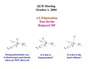
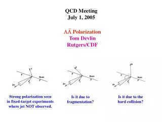
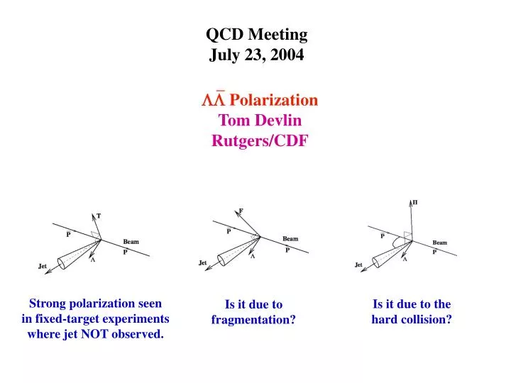
_ Polarization Tom Devlin Rutgers/CDF Strong polarization seen in fixed-target experiments where jet NOT observed. Is it due to the hard collision? Is it due to fragmentation? QCD Meeting July 23, 2004
Asymmetry plots in beam- and beam-K system (ignores jets) Polarization allowed under parity conservation is in the y-direction (second from top). Solid lines: Data Dashed lines: 20 hybrid MC-events/real-event scaled by 1/20
How Do We Get Polarization From This? • These cos() plots contain: • The Signal: and • Ks Background • Background from random 2-track crossings. __ Monte Carlo Simulation and and Ks are straightforward and in place Now working on random 2-track crossings __
Work in Progress and Planned: Summer-Fall, 2004 • Mass-constrained fits: 2-, 2-Ks, 1-ee. • Sum of weights over solutions = 1.0 per event. • Mix MC events for events with both K and solutions • as in the data, weighted by relative P(2)*P(Decay). • Further study of sailor-cowboy problem. • Add fits with mass constraints displaced by 20 MeV. • Background subtraction. • Decide whether analysis is viable or not. • If so, do polarization in the other two coordinate systems. Additional Tasks • Use 2= 2(MassConstraint) - 2(NoMassConstraint) • Random 2-track crossings.
24 : Fit with mass-constraint – 4 deg. freedom 23 : Fit without mass-constraint – 3 deg. freedom Irrelevant Fluctuations in 2 e.g. deviations from exact 3-D intersection at vertex tend to cancel. Strong deviations from correct mass DO NOT cancel in 2.
Repeat for Mass Constraint = M 20 MeV (Note that p threshold is only 38 MeV below M)
Subtract sum of two sidebands from Signal+Background (Sideband normalization used here is from previous graphs.)
Problem: The backgrounds from sidebands populate the cos plots at different values from real backgrounds. Alternate Approach: Generate hybrid MC backgrounds • For each real event, generate 20 MC events • at same decay vertex as real event • parent mass from background mass distribution • random angles in CM system • apply standard acceptance cuts • apply tight cuts in 2
Fit with no Mass Constraint: Assume Daughters are p Subtract signal, Smooth Remainder (5-bins)
Normalize Probability Distribution P(M) to Unit Area. Numerically Integrate. Find values of M(p) at intervals of 0.01 in the integral and form a table of its integral. Choose a random number R(0:1) Table Lookup and Interpolate to get M(p)
Status and Plans Three known contributions to dataset: -- Signal -- Ks Background -- Continuum 2-track background MC code exists to generate first two. Coding in progress for the third. Plan: Generate 20 MC of each type for each real event. Mix three MC samples, in appropriate proportions to produce 20 MC events for each real event. Adjust proportions of each and assumed polarization of MC ’s to fit data.