Download
1 / 20
200 likes | 203 Views
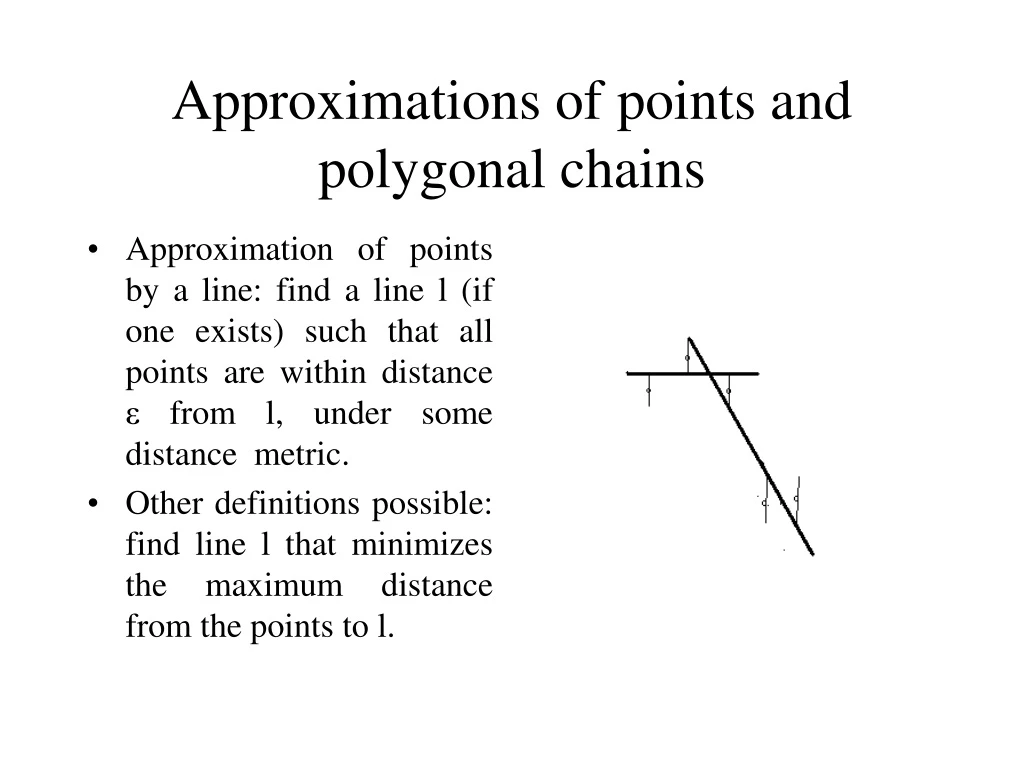
Approximations of points and polygonal chains. Approximation of points by a line: find a line l (if one exists) such that all points are within distance ε from l, under some distance metric. Other definitions possible: find line l that minimizes the maximum distance from the points to l.

E N D
Approximations of points and polygonal chains • Approximation of points by a line: find a line l (if one exists) such that all points are within distance εfrom l, under some distance metric. • Other definitions possible: find line l that minimizes the maximum distance from the points to l.
Distance Metrics • Uniform metric (prev. slide). • yi-f(xi) ≤ ε • Euclidean metric. • L1 and L∞ metrics. • Other measures possible (will be introduced latter).
Approx. of points by line • Each vertical line segment maps to a parallel strip in a dual point/line space (duality transform, to be explained shortly). • Can define the strip as intersection of two halfplanes. • Then solve a 2-D linear programming (LP) problem, which takes O(n) time.
Approx. points by min-# chain • Would a simple Greedy algorithm work? • Stab as many as possible, discard them and repeat.
Greedy vs. Dynamic Programming • If objects are convex and disjoint, O(n) time greedy algorithm is possible (vertices are unrestricted, that is, can lie anywhere). • For intersecting objects, dynamic programming gives O(n2) and O(n2 log n) time, depending on how visiting order of objects is defined.
Min-# vs. Min-ε • Min-#: given some error bound, minimize number of vertices of approximating path. • Min-ε: minimize the error of an approximating path that has at most a specified number of vertices, m (m < n). • If finite set of possible approximation errors, and if set can be computed in reasonable time, then can use min-# to solve min-ε.
Points vs. Chains • Define a piecewise linear region associated with the input, as in figure. • May ask approximating path stays in that region, for chains. • Chains may be monotone (functions) or not.
Min-# for Piecewise Linear Function • Approximation must stay in error region. • Approximation sought: monotone polygonal line with min-# of vertices. • Use “edge visibility” concept. • A point u of polygon P is visible from edge e, if there is point v on e such that line segment uv is contained in P. • An edge e’ is visible from e if there is a point of e’ visible from e. • Visibility polygon VP(P,e): points of P visible from e.
Visibility: VP(P,e) • VP(P,e) splits the polygon in a few connected regions: • Visible region/polygon; • Invisible polygons. • Consider the invisible polygon P’ that contains end point of chain. • Common boundary of P and P’ is a line segment called “window”. • Use “convex hull” algorithm to find windows. • Results in O(n) time algorithm.
Error criteria for chains • E1: Tolerance zone. • E2: Parallel-strip (also called “infinite beam”). • E3: Parallel rectangle: half of min. width of rectangle containing pk, i≤ k≤ j, with parallel sides orthogonal on line segment pipj. • E4: Rectangle: required only contain pk, i≤ k ≤j.
General Approach Using Graphs • Given: C=p1p2…pn, polygonal chain. • Directed graph G(C): • Vertex vi corresponds to point pi. • Edge (vi,vj) has weight = error of segment pipj. • For given error bound ε: G(C,ε): • Subgraph of G with edge weights ≤ ε. • A path in G(C,ε): corresponds to approximating curve with error at most ε. • Approximating curve for min-#: • Shortest path from v1 to vn in G(C,ε) (length is # arcs). • Use BFS to find it. • Min-ε: minimize ε such that in G(C,ε) there is path with at most a specified # of vertices.
Complexity • If G(C) can be computed in f(n) time: • Min-# can be solved in O(f(n)+n2) time. • Min-ε can be solved in O(f(n)+n2 log n) time. • If G(C,ε) can be computed in g(n) time: • Min-# can be solved in O(g(n)+n2) time. • Most of known solutions use this approach (see solution on handout paper for some exceptions). • The “closed” min-# and min-ε problems can eventually be solved by solving n “open” problems (better in some cases; depends on restrictions).
Complexities • Under error criteria discussed: • e1: O(n2) and O(n2 log n) time, O(n) space. • Constructs G(C,ε). • Makes use of binary search with less space. • e2: O(n2 log n) time, O(n) and O(n2) space. • Constructs G(C). • O(n2) possible if some condition holds. • Even o(n2) possible if that condition holds. • e3: O(n2 log n) time, O(n2) space (O(n) space possible?!). • Constructs G(C). • e4: O(n log n) time, O(mn log n log (n/m)) space.
Min-# under E4 • Property: In G(C,ε), if (vi,vj) є G, then (vk,vl) є G, i ≤ k < l ≤ j. • Algorithm 1: • v=1; i(1)=1; • i(v+1)=max{j | (vi,vj) є G(c,ε)}; • if i(v+1)==n then done; else v=v+1; return to 2. • The algorithm is greedy.
E4 (cont.) • There is a rectangle of width w that covers a set V of points such that it contains an edge of CH(V). • W(i,j): min. width of rectangle covering V. • For e є CH(V): • Antipodal point: point v of CH(V) farthest from line containing e. • d(e): distance from v to line containing e. • W(i,j)=min{d(e) | e is on CH(i,j)}. • Given CH(V), can find antipodal points of all edges in O(|V|) time.
E4 (cont.) • Algorithm 1’: • v=1; i(1)=1; • i(v+1)=max{j | i(v) < j ≤ n, W(i(v),j) ≤ w}; • if i(v+1)==n then done; else v=v+1; go to step 2. • Step 2 is main step. • Will show for v=1 van be executed in O(i* log i*) where i*=i(2).
E4 (cont.) • W(1,j) nondecreasing in j: use doublingbinary search to find i*. • Find m, l such that W(1,m) ≤ w, W(1,l) > w and m < l ≤ min{2m,n} • Start with m=1, l=2; double each until holds. • i* lies between m and l-1. • Again binary search to find i*:
E4 (cont.) • Algorithm 2: • k=m; l=l-1; Construct and keep CH(1,k); • h=(k+l)/2; Construct CH(k+1,h); Construct CH(1,h) from CH(1,k), CH(k+1,h); Compute wh=W(1,h); • If wh≤ w then k=h; else l=h-1; If k==l then i*=k and done; else keep CH(1,k) and go to step 2.
E4 (cont.) • Algorithm 1’+2 takes O(n log n). • Compute W(1,2g), g=1,2,..,M+1, M=log m. • W(1,j) can be found in O(j log j). • O(Σ2glog2g)=O(i*logi*). • Note that m=O(i*). • Step 2 in Alg. 2 takes O(i*logi*) • CH(1,h): O(h) (from CH(1,k) and CH(k+1,h); • W(1,h): O(h) time; • In g-th iteration CH(k+1,h) is on at most m2-g=2M-g points: O(2M-glog2M-g) time. • Executed at most M times (g=1,…M):O(Σ2M-glogM-g)=O(i*logi*).
Min-ε under E4 • O(mn(log n)(log n/m) time. (outputsensitive). • Algorithm 3 (compute min. width w*). • M’=m; i=1; w=0; • Find j, by doubling binary search, such that • i < j ≤ n, • pi,…,pn cannot be covered by m’ or fewer rectangles with width less than W(i,j), • pi,…,pn can be covered by m’ or fewer rectangles with width less than W(i,j+1). • i=j; m’=m-1; w=max{w,W(i,j)}; If i=n done; else go to step 2. • Note: in a sequence of rectangles with width w* found by min-#, the first rectangle cover points p1,…,pj, where j is found in first execution of step 2 above (then induction).