Download
1 / 37
370 likes | 475 Views
Alan Weinstein, Caltech For the LSC Burst ULWG LIGO PAC14 May 6, 2003 G030267-00-Z. Outline: Bursts: what are we looking for? Burst waveforms Burst search goals S1 data quality, final dataset Data processing pipeline Event Trigger Generators (ETG’s) Vetoes Coincidences and backgrounds

E N D
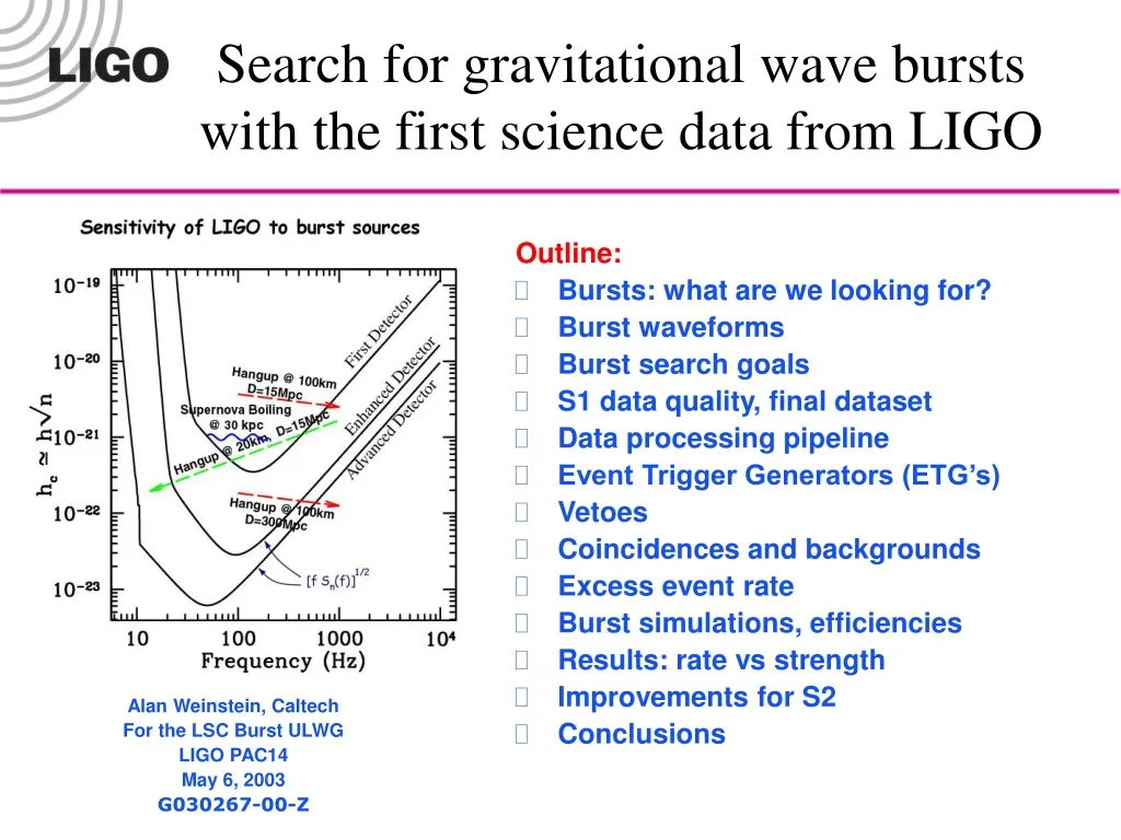
Alan Weinstein, Caltech For the LSC Burst ULWG LIGO PAC14 May 6, 2003 G030267-00-Z Outline: Bursts: what are we looking for? Burst waveforms Burst search goals S1 data quality, final dataset Data processing pipeline Event Trigger Generators (ETG’s) Vetoes Coincidences and backgrounds Excess event rate Burst simulations, efficiencies Results: rate vs strength Improvements for S2 Conclusions Search for gravitational wave bursts with the first science data from LIGO
Executive summary for S1 analysis (learning curve) • Search for short (3 -100 msec) bursts of in-band “excess power” • Require triple coincidence (H1,L1,H2) • Aim for upper limit; not ready to have confidence in detection • Require quiet, well-understood data (small fraction of S1) • Use two different burst detection algorithms • Consider, but in the end don’t use (for S1), instrumental vetoes • See a handful of events • Estimate random coincidences; roughly consistent with observed in-time coincidences. • Use Feldman-Cousins to determine upper limit on burst rate • Estimate efficiency as function of burst strength, for simple waveforms • Present results as rate-vs-strength curve • S1 “technical” paper is close (week or 2?) to release to LSC. • Long list of improvements for S2!
Bursts: what are we looking for? Gravitational waves • We look for short-duration GW bursts from SN’s, GRB’s, the unknown – whatever the cosmos throws at us! • Unlike the other LIGO S1 searches, our “signal” is ill-defined; waveforms unknown or untrustworthy – a menagerie!
Zwerger-Müller SN waveforms • astrophysically-motivated waveforms, computed from simulations of axi-symmetric SN core collapses. • Almost all waveforms have duration < 0.2 sec • A “menagerie”, revealing only crude systematic regularities. Inappropriate for matched filtering or other model-dependent approaches. • Their main utility is to provide a set of signals that one could use to compare the efficacy of different filtering techniques. • Absolute normalization/distance scale.
Bursts: time-frequency character Damped sinusoid merger chirp ringdown ZM SN burst • We aim to be sensitive to bursts with generic t-f properties: • longish-duration, small bandwidth (ringdowns, Sine-gaussians) • longish-duration, large bandwidth (chirps, Gaussians) • short duration, large bandwidth (BH mergers) • In-between (Zwerger-Muller or Dimmelmeier supernova simulation waveforms)
Ad-hoc signals: (Sine)-Gaussians SG 554, Q = 9 These have no astrophysical significance; But they are well-defined in terms of waveform, duration, bandwidth, amplitude; They can constitute a crude “basis set” to “span” the detection band If our algorithms can detect these, they can detect any waveform with similar duration, bandwidth, amplitude
Burst search goals • Search for short-duration bursts with unknown waveforms • Short duration: < 1 second; more typically, < 0.2 seconds. • Matched filtering techniques are appropriate for waveforms for which a model exists. Hard to be sure they won’t miss some unknown waveform. Explicitly exclude, here! • Instead, focus on excess power or excess oscillation techniques • Although the waveforms are a-priori unknown, we must require them to be in the LIGO S1 sensitivity band (~ 150-3000 Hz) • Search for gravitational wave bursts of unknown origin • Bound on the rate of detected gravitational wave bursts, viewed as originating from fixed strength sources on a fixed distance sphere centered about Earth, expressed as a region in a rate v. strength diagram. • Search for GW bursts associated with gamma-ray bursts (GRB’s) • The result of this search is a bound on the strength of gravitational waves associated with gamma-ray bursts. • Work in progress – not reported on today!
Gamma Ray Bursts during S1and LIGO coverage Focus on HETE-2 detector (good directional info, for LIGO coincidence)
Detection Confidence • Multiple interferometers – coincidence! • Three interferometers within LIGO (H1 = LHO-4K; H2 = LHO-2K; L1 = LLO-4K) • GEO data were analyzed in parallel, but not taken to the end; not included in S1 paper! • No use yet made of double-coincidences, or triple coincidences with 4 detectors… • Timing accuracy of ~ 100 usec (16 kHz digitization); 10 msec light travel time between LHO/LLO • Veto environmental or other instrumental noise • Veto time coincidences with bursty glitches in environmental channels (seismic, acoustic, E-M, …) which are known to feed into GW channel • Bursty glitches in auxiliary interferometer channels (eg, PSL, or SymPort signals), which can feed into GW channel, but which would not respond measurably to a real GW signal • Detection computation • Efficient filters for model-able signals • As tight a time-coincidence window as possible • Consistency amongst burst signals from multiple detectors, in amplitude, frequency band, waveform • Data quality is really important in this analysis!
Detection Confidence (?) • DETECTIONrequires: • well understood detector: • Minimal and stationary burstiness • stationarity of noise • (and good sensitivity!) • well understood, tuned and tested, data processing algorithms and procedures. • Clearly established criteria for establishing confidence in real GW signal • NONE of these were firmly in place for S1 • estimate background rate • quote upper limits.
S1 Data Statistics 170hours L1 235hours H1 298hours H2 All 3 96hours 17 days = 408 hours
Playground data • Search algorithms require tuning! • Avoid bias: use playground data. • We chose a representative sample of 13 locked segments, from the triple coincidence segments. They add up to 9.3 hours. • All tuning of ETG and veto trigger thresholds done on playground data only. • Choose threshold: Aim for Order(1) accidental coincidences in full S1 • We do not include these 9.3 hours in the full analysis and results.
Non-stationarity, and Epoch Veto • BLRMS noise in GW channel is not stationary. • Detector response to GW (calibrated sensitivity) is not stationary. • Bursty-ness of GW channel is not stationary. • Fortunately, these varied much less in S1 than in E7, thanks to efforts of detector and DetChar groups. • Much of this is driven by gradual misalignment during long locked stretches. • Under much study!
Stationarity of noise: BLRMS • BLRMS noise is far from stationary. • Playground data (pink vertical lines) are not very representative. • We veto certain epochs based on excessive BLRMS noise in some bands.
Time-dependence of calibration:Monitoring calibration lines C(f) is sensing function;H(f) is open-loop-gain 51.3 972.8 Veto epochs with no, or low a. Require calibration line present and strong! Did not anticipate this…
Final dataset for analysis • S1 run: 408.0 hours • 3 IFOs in coincidence: 96.0 hours • Set aside playground: 86.7 hours • Granularity in pipeline (360 sec): 80.8 hours • Epoch veto: 54.6 hours • Keep only well-calibrated data: 35.5 hours
Data processing pipeline • Event trigger: indicator of grav. wave event (SLOPE, TFCLUSTERS) • LDAS: LIGO Data Analysis System • Auxiliary channels: indicator of instrumental or environmental artifacts • DMT: Data Monitoring Tool (part of Global Diagnostic System) • IFO trigger: event triggers not vetoed (ROOT, Matlab) • Vetoes eliminate particularly noisy data (6 minute epoch averages) • Coincident events: “simultaneous” IFO triggers (ROOT, Matlab) • Time window: maximum of {light travel time between detectors, uncertainty in signal arrival time identification} • Frequency window for TFCLUSTERS
Data flow in LDAS User pipeline request • frameAPI • datacondAPI • mpiAPI • wrapperAPI • LAL code • eventmonAPI • metadataAPI • metaDB
Data conditioning in datacond • All of our burst filters are expected to work best with (at least, approximately) whitened data. • This is not matched filtering: don’t need to know detector response function to find excess power. • In datacondAPI, we (approximately) whiten and HP (at 150 Hz) the data with pre-designed linear filters. • New filters with better performance are under design. • No attempt (yet) at line removal: but we believe that this will eventually be very necessary.
Event Trigger Generators • Three LDAS filters (ETG’s or DSOs) are now being used to recognize candidate signals: • POWER - Excess power in tiles in the time-frequency plane • TFCLUSTERS - Search for clusters of pixels in the time-frequency plane. • SLOPE - Time-domain templates for large slope or other simple features • However, the POWER ETG was not well optimized in time for this analysis, and technical problems forced it to be set aside. • The SLOPE and TFCLUSTERS ETG’s performed reasonably well in this analysis, but it is clear that they both could have been better tuned and optimized • For this analysis, use SLOPE and TFCLUSTERS as-is, no claim of optimal performance. • These ETG’s generate event triggers that indeed correspond to bursts of excess power; and provide an (uncalibrated, waveform-dependent) measure of the energy in the burst • Both ETG’s required whitened, HPF’ed data. This pre-filtering also lacked careful optimization, and can certainly be improved. • NEW filters under development! • Multi-detector coherence, matched filtering, wavelets, non-stationarity detectors… • We have more implemented algorithms than time to evaluate them: an embarrassment of riches!
tfclusters • Compute t-f spectrogram, in 1/8-second bins • Threshold on power in a pixel, get uniform black-pixel probability • Simple pattern recognition of clusters in B/W plane; threshold on size, or on size and distance for pairs of clusters
Veto Channels • look for glitches on many different channels • correlated in time with GW channel glitches • would not have registered real GW’s • significantly reduce single-IFO background burst rate, while producing minimal deadtime • PEM channels not observed to be useful; filtering of environmental noise works well! • IFO channels: In contrast to E7, no auxiliary channel vetoes were found to be very efficacious with S1 data. • This is good! The most promising auxiliary channels were the ones most closely coupled with the GW (AS-Q) channel: AS-I, SP-I, SP-Q, MICH-CTRL. • This is too close for comfort! Further study is required before such vetoes can be safely and confidently employed. • For this analysis, NO vetoes on auxiliary channel bursts! • LSC-AS_Q (GW channel) • LSC-AS_I • LSC-REFL_Q • LSC-REFL_I • LSC-POB_Q • LSC-POB_I • LSC-MICH_CTRL • LSC-PRC_CTRL • LSC-MC_L • LSC-AS_DC • LSC-REFL_DC • IOO-MC_F • IOO-MC_L • PSL-FSS_RCTRANSPD_F • PSL-PMC_TRANSPD_F
Cuts on coincident event triggers • Choose lowest practical trigger thresholds, maximizing our sensitivity, at the cost of fake coincidences. • Rely heavily on triple coincidence to make the fake rate manageable! • Might optimize differently if our goal is detection, not upper limit. • Require temporal coincidence: trigger windows (start time, duration) must overlap within coincident window. • tfclusters ETG (currently) finds clusters in t-f plane with 1/8 second time bins • can’t establish coincidences to better than that granularity. • Currently, coincidence window for tfclusters triggers is 500 msec. • tfclusters also estimates frequency band; require consistency • slope ETG has no such limitation • currently, coincidence window for slope triggers is 50 msec. • slope does not yet estimate frequency band • More work required to tighten this to a fraction of 10 msec light travel time between LHO/LLO. • No cut, yet, on consistency of burst amplitude (calibrated), or waveform coherence. These are an essential next step!!
Background: Accidental coincidence rate • Determine accidental rate by forming time-delayed coincidences • Trigger rate is non-stationary, and triggers can extend over 1-8 secs. Carefully choose time lag steps, windows: calculated with 24 lags (8 sec steps, -100 to + 100 sec). Background rate is reasonably Poissonian. • Correlated noise between H1 and H2? Study accidental rate using LHO-LLO time lag, keeping H1&H2 in synch. tfclusters slope
Coincident events, estimated background, excess event rate and UL • Combine the observed coincident event rate with the background estimate and its uncertainty • Use the Feldman-Cousins technique for establishing confidence bands for counting experiments in the presence of background (a standard technique in HEP) • Marginalize over uncertainty in the background rate. • The statistical uncertainty is small because of many independent time lags. Searched for, and found no evidence for systematic bias in estimate of background rate. • The marginalization over the background rate uncertainty has insignificant effect on the limits • Note: if we had zero signal and zero background, the 90% CL upper limit would be 2.44 events
Burst Simulations - GOALS • Test burst search analysis chain from: • IFO (ETM motion in response to GW burst) • GW channel (AS_Q) data stream into LDAS • search algorithms in LDAS • burst triggers in database • post-trigger analysis (optimizing thresholds and vetoes, clustering of multiple triggers, forming coincidences) • Evaluate pipeline detection efficiency for different waveforms, amplitudes, source directions, and different algorithms (ETGs) • Tune ETG thresholds and parameters (playground data only!) • Figure of merit: minimize background rate / efficiency • Compare simulated signals injected into IFO with signals injected into data stream: make sure we understand IFO response
Efficiency for injected signals • Generate a digitized burst waveform h(t)(in this example, SG554 with varying hpeak) • Filter through calibration (strain AS_Q counts) • Add to raw AS_Q data, sampling throughout S1 • Pre-filter and pass to ETG, as usual • Look for ETG trigger coincident with injection time • Repeat many times, sampling throughout S1 run • Average, to get efficiency for that waveform, amplitude, IFO, ETG combo • Deadtime due to vetoes not counted in efficiency • Can also evaluate triple coincidence efficiency, assuming optimal response of all 3 detectors (unrealistic) – black curve. • Note that ETG power (on which we threshold) tracks input peak strain amplitude well. • ETG power is a very ETG-specific quantity; not directly related to GW energy or hpeak. • Nonetheless, it tracks hpeak , for a fixed waveform. • true for all ETG’s, even slope.
Sine-Gaussians:root-sum-square “hrss” at 50% efficiency (strain/Hz-1/2)
Averaging over source direction and polarization • Generate single-IFO efficiency curve vs signal amplitude, assuming optimal direction / polarization. • Different for each data epoch • Different for each IFO • Different for each waveform. • Different for each ETG / threshold • Assuming source population is isotropic, determine single-IFO efficiency versus amplitude, averaged over source direction and polarization, using single-ifo response function. • This is easily accomplished with simple Monte Carlo; no need to go back to detailed LDAS simulations. • But, this is wrong, if both polarizations are present, with different waveforms.
Coincidence efficiency, averaged over source direction & polarization • Efficiency for coincidences is the product of single-IFO efficiencies, evaluated with the appropriate response of each IFO to GWs of a given source direction / polarization. • This assumes that detection is a random event, uncorrelated between detectors. • Easily accomplished with simple Monte Carlo, using knowledge of detector position and orientation on Earth. No need to go back to detailed LDAS simulations. • Must estimate any additional loss of efficiency due to post-coincidence event processing (for S1, this is negligible). • Check against coincident simulations, including ±10 msec time delay.
Coincident efficiency vs hrss for different waveforms, ETGs slope tfclusters For these waveforms, tfclusters wins by a nose; but both ETG’s need better tuning!
Result: rate vs strength • tfclusters detects less than 1.4 events/day at 90% CL • Divide by efficiency curve for a particular waveform, to get rate vs strength exclusion region • 20% uncertainty in calibration (strain counts);choose conservative right-most band • Repeat, for each waveform and ETG
Results, for tfclusters and slope tfclusters slope
The S2 Run • Eight-week run February 14 - April 14 2003 • Detector sensitivities are much better than for S1 • Duty factors are about the same • Improvements in stability since S1: • Better alignment control, especially for H1 • Better monitoring in the control rooms • Fewer episodes of greatly increased BLRMS noise in GW channel • Careful attention to calibration lines, monitoring • Burst and inspiral search codes ran in near-real-time for monitoring purposes • With improved noise and stability, will burstiness be better or worse than S1? Under study!
Improvements for S2 S1 analysis leaves MUCH room for improvement for S2 and beyond! • GW channel prefiltering (HPF, whitening, basebanding?) needs optimization • ETG’s need careful tuning and optimization for best efficiency / fake rate • Choice of thresholds, clustering of multiple triggers associated with one event • Minimize loss of useful data associated with epoch and calibration vetoes • Find and employ effective and safe vetoes on auxiliary channels; quantify cross-coupling to and from GW channel • Post-coincidence processing: Go back to raw data! • Determine trigger start time to sub-msec precision • Determine calibrated peak amplitude, require consistency • Determine signal bandwidth, require consistency • Determine cross-correlation between coincident waveforms and require consistency • Make use of double coincidences • Incorporate GEO, TAMA, VIRGO
More improvements • More, and better motivated, simulations • Establish clear method to translate results to arbitrary burst waveforms • Limits for astrophysically-motivated waveforms(Zwerger-Müller, DFM, others…?) • More detailed studies of cross-couplings, calibration, and simulations, using hardware injections • Fully coherent approach: WaveBurst • Matched filtering: choice of basis set. • “Delta functions” as in bar detectors • Sine-gaussians with varying Q. • Establish well-defined criteria for detection! • The “inverse” problem: determine waveform associated with detected event, location in sky, quasi-realtime alert to telescopes • Sidereal time distribution of events (galactic disk) • Targeted upper limits (galactic center, disk)
Conclusions • The S1 burst analysis is a first step towards full exploitation of the LIGO detectors for discovery of GW bursts • The resulting limits are weak, not easy to interpret, and not of astrophysical interest… • BUT, we know how to improve these things! • Moving on to S2, and discovery!