Download
1 / 24
240 likes | 379 Views
Bunched-Beam Phase Rotation- Variation and 0ptimization. David Neuffer, A. Poklonskiy Fermilab. Talk Intro. “Proprietary” documents: http://www.cap.bnl.gov/mumu/study2a/. 0utline. Introduction Study 2 Study 2A “High-frequency” Buncher and Rotation Concept

E N D
Bunched-Beam Phase Rotation-Variation and 0ptimization David Neuffer, A. Poklonskiy Fermilab
Talk Intro “Proprietary” documents: http://www.cap.bnl.gov/mumu/study2a/
0utline • Introduction • Study 2 Study 2A • “High-frequency” Buncher and Rotation • Concept • Matched cooling channel • Study 2A scenario • Match to Palmer cooling section • Obtains up to ~0.2 /p • Variations • Be absorber (or H2, or …) • Shorter rotator (52m 26m), fewer rf frequencies • Short bunch train (< ~20m) • Optimization ….
R&D goal: “affordable” e, -Factory • Improve from baseline: • Collection • Induction Linac “high-frequency” buncher • Cooling • Linear Cooling Ring Coolers(?) • Acceleration • RLA “non-scaling FFAG” – e– + ne + and/or + e+ + n + e
Study 2 system • Drift to develop Energy- phase correlation • Accelerate tail; decelerate head of beam (280m induction linacs (!)) • Bunch at 200 MHz • Inject into 200 MHz cooling system Em ctm
Adiabatic buncher + Vernier Rotation • Drift (90m) • decay; beam develops correlation • Buncher(60m)(~333200MHz) • Forms beam into string of bunches • Rotation(10m)(~200MHz) • Lines bunches into equal energies • Cooler(~100m long)(~200 MHz) • fixed frequency transverse cooling system Replaces Induction Linacs with medium-frequency rf (~200MHz) !
Adiabatic Buncher overview • Want rf phase to be zero for reference energies as beam travels down buncher • Spacing must be N rf rf increases (rf frequency decreases) • Match torf= ~1.5m at end of Rotator • Gradually increase rf gradient (linear or quadratic ramp): Example: rf : 0.90~1.4m Captures both (+, -)
Rotation • At end of buncher, change rf to decelerate high-energy bunches, accelerate low energy bunches • Reference bunch at zero phase, set rf less than bunch spacing (increase rf frequency) • Places low/high energy bunches at accelerating/decelerating phases • Can use fixed frequency or • Change frequency along channel to maintain phasing • “Vernier” rotation –A. Van Ginneken Z(N) – Z(0) = (N + δ) λrf(s) rf : ~1.41.5m in rotation; Nonlinearities cancel: T(1/) ; Sin()
Key Parameters • General: • Muon capture momentum (200MeV/c?) 280MeV/c? • Baseline rf frequency (200MHz) • Drift • Length LD • Buncher– Length (LB) • Gradient VB (linear OK) • Rf frequency: (LD + LB(z)) (1/) =RF • Phase Rotator-Length (LR) • Vernier, offset : NR, V • Rf gradient VR • COOLing Channel-Length (LC) • Lattice, materials, VC, etc. • Matching …
Study 2a Cooling Channel • Need initial cooling channel • (Cool T from 0.02m to 0.01m) • Longitudinal cooling ? • Examples • Solenoidal cooler (Palmer) • “Quad-channel” cooler • 3-D cooler • Match into cooler • Transverse match • B=Const. B sinusoidal • Gallardo, Fernow & Palmer
Palmer Dec. 2003 scenario • Drift –110.7m • Bunch -51m • V’ = 3(z/LB) + 3 (z/LB)2 MV/m (× 2/3) (85MV total) • (1/) =0.0079 • -E Rotate – 52m – (416MV total) • 12 MV/m (×2/3) • P1=280 , P2=154V = 18.032 • Match and cool (100m) • V’ = 15 MV/m (× 2/3) • P0 =214 MeV/c • 0.75 m cells, 0.02m LiH
Study2AP June 2004 scenario • Drift –110.7m • Bunch -51m • V(1/) =0.0079 • 12 rf freq., 110MV • 330 MHz 230MHz • -E Rotate – 54m –(416MV total) • 15 rf freq. 230 202 MHz • P1=280 , P2=154V = 18.032 • Match and cool (80m) • 0.75 m cells, 0.02m LiH • “Realistic” fields, components • Fields from coils • Be windows included
Simulation of Study 2Ap Drift (110m) Bunch (162m) E rotate (216m) Cool (295m) System would capture both signs (+, -) !!
Variation –Be absorbers • Replace LiH absorbers with Be absorbers • suggested by M. Zisman • (0.02m LiH 0.0124m Be) • Performance somewhat worse • Cooling less (tr ~0.0093; LiH has 0.0073) • Best is ~0.21/p within cuts after 80m cooling • (where LiH has ~0.25 at 100m) • Be absorbers could be rf windows • H2 gas could also be used • Gas-filled cavities (?)
Shorter bunch Rotator • Drift –123.7m (a bit longer) • Bunch -51m • V’ = 3(z/LB) + 3 (z/LB)2 MV/m • (1/) =0.0079 • -E Rotate – 26m – • 12 MV/m (× 2/3) • P1=280 , P2=154V = 18.1 • (Also P1=219 , P2=154, V = 13.06) • Match and cool (100m) • V’ = 15 MV/m (× 2/3) • P0 =214 MeV/c • 0.75 m cells, 0.02m LiH • Obtain ~0.22 /p
Try with reduced number of frequencies • Change frequency every 6 cells (4.5m) • Buncher (11 freqs.): • 294.85, 283.12, 273.78, 265.04, 256.04, 249.13, 241.87, 235.02, 228.56, 222.43, 216.63 MHz • Rotator (6 freqs) • 212.28, 208.28, 205.45, 203.52, 202.34, 201.76 • Cooler(200.76 MHz) • Obtains ~0.2 /p • (~0.22 /p for similar continuous case - 105 frequencies) • Not reoptimized …. • Phasing within blocks could be improved, match into cooling…
Short bunch train option • Drift (20m), Bunch–20m (100 MV) • Vrf = 0 to 15 MV/m ( 2/3) • P1 at 205.037, P2=130.94 • N = 5.0 • Rotate – 20m (200MV) • N = 5.05 • Vrf = 15 MV/m ( 2/3) • Palmer Cooler up to 100m • Match into ring cooler • ICOOL results • 0.12 /p within 0.3 cm • Could match into ring cooler (C~40m) (~20m train) 40m 60m 95m
FFAG-influenced variation – 100MHz • 100 MHz example • 90m drift; 60m buncher, 40m rf rotation • Capture centered at 250 MeV • Higher energy capture means shorter bunch train • Beam at 250MeV ± 200MeV accepted into 100 MHz buncher • Bunch widths < ±100 MeV • Uses ~ 400MV of rf
Lattice Variations (50Mhz example) Example I (250 MeV) • Uses ~90m drift + 100m 10050 MHz rf (<4MV/m) ~300MV total • Captures 250200 MeV’s into 250 MeV bunches with ±80 MeV widths Example II (125 MeV) • Uses ~60m drift + 90m 10050 MHz rf (<3MV/m) ~180MV total • Captures 125100 MeV’s into 125 MeV bunches with ±40 MeV widths
Variations, Optimizations • Shorter bunch trains ? (for ring cooler, +-- collider: more ’s lost?) • Longer bunch trains (more ’s, smaller E) • Remove/reduce distortion ? • Different final frequencies (200,88,44Mhz?) • Number of different RF frequencies and gradients (6010 ok?) • Different central momenta (200MeV/c, 300MeV/c …?) • Match into cooling channel, accelerator • Transverse focusing (solenoidal field?) • Mixed buncher-rotator? • Cost/perfomance optimum
Control Theory Approach A. Poklonskiy - MSU - impulse effect model or - continuous model u– control function (incorporate lattice parameters) - quality functional Seek for usuch that it will minimize (maximize) some functional of this type describing some properties of the beam we want to maintain during its propagating through the lattice (1st part) and at the end (2nd part). is the set of coordinates of the beam particles at the time tunder control functions u
Control Theory Approach A. Poklonskiy - MSU T E central t If we define penalty functions on a rectangle as and the quality functional we can perform optimization using control theory methods (gradient?)
A. Poklonskiy - Summary • Model of buncher and phase rotator was written in COSY Infinity • Simulations of particle dynamics in lattice with different orders and different initial distributions were performed • Comparisons with previous simulations (David Neuffer’s code, ICOOL, others) shows good agreement • Several variations of lattice parameters were studied • Model of lattice optimization using control theory is proposed
Summary • High-frequency Buncher and E Rotator simpler and cheaper (?) than induction linac system • Performance better (?) than study 2, And • System will capture both signs (+, -) ! (Twice as good ?) • Good R&D model for +-- Collider. • Method could be baseline capture and phase-energy rotation for anyneutrino factory … To do: • Optimizations, Best Scenario, cost/performance …