Download

1 / 22
220 likes | 294 Views
Spreadsheet-based 0ptimization. With modern spreadsheets, optimization is a snap. Objective: Execute the optimization of profit functions using the Excel spreadsheet. Problem : Maximizing profits from the sale of microchips. Our inverse demand function for microchips [ 1 ] :.

E N D
Spreadsheet-based 0ptimization With modern spreadsheets, optimization is a snap Objective: Execute the optimization of profit functions using the Excel spreadsheet.
Problem : Maximizing profits from the sale of microchips Our inverse demand function for microchips [1]: P = 170 – 20Q The Revenue (R) function is given by: R = P · Q = (170 – 20Q)Q = 170Q – 20Q2 Thus marginal revenue (MR) is given by dR/dQ = 170 –40Q
The cost function (C) is given by [2] C = 100 + 38Q Thus the marginal cost (MC) function is given by: dC/dQ = 38 The profit () function is given by: R – C = 170Q – 20Q2 –(100 + 38Q) = 132Q – 20Q2 –100 Thus the marginal profit function (M) is given by: d /dQ = 132 – 40Q
Step 3: Move your cursor to cell c7 and type the following in the formula bar: =170-20*b7 Hit “enter” or click right on the green check mark to the left of the formula bar. Now your spreadsheet should look like this:
Step 4: Move your cursor to cell d7 and type the following in the formula bar: =b7*c7 Hit “enter” or click right on the green check mark to the left or the formula bar. Now your spreadsheet should look like this:
Step 5: Move your cursor to cell e7 and type the following in the formula bar: =100+38*b7 Hit “enter” or click right on the green check mark to the left or the formula bar. Now your spreadsheet should look like this:
Step 6: Move your cursor to cell f7 and type the following in the formula bar: =d7-e7 Hit “enter” or click right on the green check mark to the left or the formula bar. Now your spreadsheet should look like this:
3 ways to maximize profits () Now we will show you 3 methods of maximizing the profit function using Excel.
Method 1: Change the value of the number in cell b7 until you find the highest corresponding value in cell f7. Example: Enter the number “3.0” in cell b7. Notice that profit increases to 116.
Method 2: Use MR and MC as guides. Vary the numerical values in cell b7 until MR =MC (or alternatively, Mprofit = 0). Example: Enter the number “3.0” in cell b7. Notice that profit increases to 116.
Method 2: Use MR and MC as guides. Vary the numerical values in cell b7 until MR =MC (or alternatively, Mprofit = 0). Step 1: Type MR, MC, and Mprofit into cells d12, e12, and f12 respectively
Step 2: To compute MR when quantity is equal to 2 lots, place your cursor in cell d14 and type the following in the formula bar: =170-40*b7 Your spreadsheet should look like this:
Step 3: Note that MC = 38, so type this into cell e14.To compute marginal profit (Mprofit) move your cursor to cell f14 and type the following in the formula bar: =132-40*b7 Your spreadsheet should now look like this:
Step 4: Now adjust the numerical values in cell b7 until MR = MC, or Mprofit = 0. Example: Type “3.0” in cell b7. Your spreadsheet should now look like this:
Method 3:Use the Excel “solver” function • Move your cursor to cell f7. • From the “tools” menu select “solver”. You should see a dialog box like this: Solver Parameters Set Target Cells $F$7 Solve Equal to Max Min Close By Changing Cells: Options Subject to Constraints: Add Change Delete
Notice that the default is “Max”—that’s OK– we are trying a maximize a profit function. • In the “By Changing Cells” space type: $B$7. Remember we are seeking to find the profit maximizing output-price combination. • Now click on the “solve” button. Solver Parameters Set Target Cells $F$7 Solve Equal to Max Min Close By Changing Cells: $B$7 Options Subject to Constraints: Add Change Delete
The solver function found the profit maximizing output (3.3 lots) and price ($104,000 per lot).
Constrained optimization Suppose we are seeking to maximize profits subject to the constraint that our price per lot cannot exceed $91,000—that is:P 91
Move your cursor to cell f7 and access the “solver” dialog box from the tools menu. • Now click on the add button and you will find a dialog box (something) like this: • Type c7 into Cell Reference space and 91 into constraint space. Now click on OK Add Constraint Constraint: Cell Reference: c7 <= 91 OK Cancel Add Help Note: <= is the default, which works in our case.
The solver function found the output (4.0 lots) that maximizing profits subject to the price constraint.