Download

1 / 58
580 likes | 825 Views
Chapter 9 Competitive Markets. Learning Objectives. 1. State the key assumptions of the theory of perfect competition. 2. Show how to derive a competitive firm’s supply curve. 3. Identify whether competitive firms are making losses or profits in the short run.

E N D
Chapter 9 Competitive Markets
Learning Objectives 1. State the key assumptions of the theory of perfect competition. 2. Show how to derive a competitive firm’s supply curve. 3. Identify whether competitive firms are making losses or profits in the short run. 4. Explain the role that profits, entry, and exit play in a competitive industry’s long-run equilibrium.
9.1Market Structure and Firm Behaviour Competitive Market Structure The competitiveness of the market is related to the power individual firms have to influence market prices or the terms on which their product is sold. The less power an individual firm has to influence the market in which it sells its product, the more competitive is that market’s structure.
9.1Market Structure and Firm Behaviour Competitive Behaviour The term competitive behaviour refers to the degree to which individual firms actively vie with one another for business. For example, Petro-Canada and Esso engage in competitive behaviour but their market is not competitive. In contrast, two wheat farmers do not engage in competitive behaviour but they both exist in a very competitive market.
The Significance of Market Structure Note that the demand curve for the firm’s output may not be the same as the demand curve for the industry as a whole. The characteristics of the market — the market structure — determine the relationship between the market demand curve for the industry’s product and the demand curve that each firm in that industry faces.
The Assumptions of Perfect Competition • All the firms in the industry sell an identical (homogeneous) product. (Also assumed with oligopoly, not assumed with monopolistic competition) • Customers know the nature of the product being sold and the prices charged by each firm. • The level of the firm’s output at which its LRAC reaches a minimum is small relative to the industry’s total output. (Not assumed for monopoly, oligopoly) • Firms in the industry are free to exit and “outside” firms are free to enter. (Also assumed for monopolistic competition, not assumed for monopoly, oligopoly)
Implications of the Assumptions The first three assumptions imply that each firm is a price taker in a perfectly competitive industry. Thus, any firm can alter its level of production without affecting the market price. A firm operating in a perfectly competitive market has no power to influence the market price through its own actions. It must passively accept whatever happens to be the market price, but it can sell as much as it wants at that price. The difference between the wheat farmers and Petro-Canada is the degree of market power.
The Demand Curve for a Perfectly Competitive Firm Price Price S D (Firm) D (Mkt) Quantity (Millions of Tonnes) quantity (Thousands of Tonnes) A major distinction between firms in perfectly competitive markets and firms in any other type of market is the shape of the firm’s own demand curve. Even though the demand curve facing the entire industry is negatively sloped, each firm in a perfectly competitive market faces a horizontal demand curve (at the market price).
This is because variations in the firm’s output have no effect on price. This does not mean the firm could actually sell an infinite amount at the going price, but… that a variation in normally possible levels of production will have a negligible effect on total industry output, and consequently a negligible effect on market price. E.g., Suppose there are 1,000 firms in the industry, each producing output ‘q’, so total industry output is 1000*q. Suppose one cuts its output in half. Now, total industry output will decline to (999.5)*q. Industry output will be 99.95% of its previous level—there is a negligible effect on price; for practical purposes, price does not change.
Total, Average, and Marginal Revenue Total revenue (TR) is the total amount received by the seller from the sale of a product. If q units are sold at p dollars each, then TR = p x q. Average revenue (AR) is the amount of revenue per unit sold. It is equal to total revenue divided by the number of units sold, and is thus equal to the price at which the product is sold: AR = (p x q)/q = p. Marginal revenue (MR) is the change in the firm’s total revenue resulting from a change in its sales by one unit. In a perfectly competitive industry, the market price is unaffected by each firm’s level of output, and so the firm’s marginal revenue is equal to price (which is equal to average revenue): AR = MR = price.
Price(p) Quantity(q) TR = px q AR = TR/q MR = TR/q 3 3 3 3 10 11 12 13 30 33 36 39 3 3 3 3 3 3 3 Dollars per Unit TR Dollars 39 30 AR =MR=p 3 10 13 10 13 Output Output For a firm in perfect competition, price is always equal to marginal revenue. This is not true for monopoly firms, neither for firms in either imperfectly competitive market structure.
Profit-Maximizing Output All firms, irrespective of market structure (competitive, monopoly, imperfectly competitive) make output decisions on the same basis Two questions to answer: • Should the firm produce anything at all? • If (and only if) we answer “yes” to the first question, How much output should the firm produce?
Should the Firm Produce Anything? • If there is some output level at which total revenue received exceeds total AVOIDABLE cost of production, the firm is better off producing that output than not producing at all • In the short run, only variable cost can be avoided by not producing at all (fixed costs are borne whether or not the firm produces) • The firm produces if there is some output at which TR>TVC • Divide the previous expression by output quantity to re-express the condition as “if P>AVC”
Rules for All Profit-Maximizing Firms Should the Firm Produce at All? A firm should not produce at all if, for all levels of output, the total variable cost of producing that output exceeds the total revenue from selling it or, equivalently, if the average variable cost of producing the output exceeds the price at which it can be sold. AVC $/Unit MC p AR =MR=p Output
The price at which the firm can just cover its average variable cost, and so is indifferent between producing and not producing, is called the firm’s shut-down price. How Much Should a Firm Produce? If it is worthwhile for the firm to produce at all, the firm should produce the output at which marginal revenue (slope of Total Revenue) equals marginal cost (slope of Total Cost). A perfectly competitive firm should produce the output that equates its marginal cost of production with the market price of its product (as long as price exceeds average variable cost).
TC In a perfectly competitive industry, the market determines the price at which the firm sells its product. The firm then chooses to produce the quantity of the output that maximizes its profits. TR Dollars Profit > 0 q* 0 Output When the firm has reached the position where its profits are maximized, it has no incentive to change its output. Note that there are many flow rates of output at which positive profits are earned—but only one (q*) at which profit is maximized.
“Rule of Rational Life” • Provided the first condition is satisfied (revenue exceeds avoidable cost at some output level(s))… • The firm increases its profit if it follows “the rule of rational life” (McCloskey) • Rule is framed in terms of small (marginal) changes • If a small increase in an activity level contributes more to benefit (here, revenue) than it adds to cost, increase the activity. • If a small decrease in an activity level reduces costmore than it reduces benefit (revenue), reduce the activity
Rational Life & Profit Maximization • For a profit-maximizing firm, the rule reduces to • Increase output if associated additional revenueexceeds associated additional cost • Additional revenue called “Marginal Revenue” • Additional cost called “Marginal Cost” • Rule implies the firm should increase output if MR>MC … reduce output if MR<MC • This rule applies to (profit-maximizing) firms in all types of market structures
Profit Maximizing Output, Perfectly Competitive Firm • The marginal revenue from selling another unit, for a competitive firm… • Equals the price of that unit, which is the price of every unit • The profit maximizing output rate is that flow rate of output at which PRICE equals marginal cost • This is a special case of the general rule MR = MC
TVC TR Dollars $/Unit Profit (net of fixed cost) if output is q* MC AVC Loss if output is qL P= MR Output qL q* qL q* Output There are (or can be) TWO output levels at which P = MC, qL and q*. Why will the firm choose q*, at which MC intersects (P = MR) from below? When P = MC(right side), the slope of TVC = slope of TR. At qL, P = MC, but (left side) profit is at a minimum, not a maximum
Uses “smooth” cost function (chosen for mathematical convenience—not realism) To calculate Marginal Cost at an integer quantity, compute cost of producing ½ unit less and ½ unit more—difference in cost is very close to MC at that quantity E.g., to find MC of 12 units, compute cost of 11½ and cost of 12½ --difference is MC of 12 units MC computations are not shown in detail, but they can be made available Total cost function used was The first three terms (functions of “Q”) together describe total variable cost Final term (2,250) represents fixed cost Numerical Example
Cost Curve Diagram MC ATC Min ATC AVC Min AVC AFC
Optimal Outputs • First situation— price = $25 • Demonstration of the irrelevance of the second “rule” if the first condition is not satisfied • Increase output as long as MR (= P for a competitive firm) > MC, but… • There is no output at which total revenue (when P = 25) exceeds (or even equals) total variable cost. • Firm does better by shutting down (pays fixed cost from own pocket) since every positive output entails variable (avoidable) costs greater than total revenue —production of any positive output results in losses greater than the amount of fixed cost (unavoidable)
Revenue, Variable Cost MC ATC Loss =($291-$25)*9 = ($266)*9 = $2,394 AVC AFC Variable Cost Revenue
Optimal Outputs • Second situation—price = $40 • Increase output as long as MR (= P for a competitive firm) > MC • Optimal output (if producing at all) is 10 units • At Q=10, total revenue equals total variable cost (total avoidable cost) • Firm is likely indifferent between producing ten units and not producing at all— either way, loss exactly equals fixed cost of $2,250 • $40 is the shut-down price—firm will not produce if P < $40
Revenue, Variable Cost MC ATC Loss = ($265-$40)*10 =($225)*10 = $2,250 AVC AFC Revenue Variable Cost
Optimal Outputs • Third situation—price = $100 • Increase output as long as MR (= P) > MC • Optimal output (if producing at all) is 12 units • At Q=12, total revenue exceeds total variable cost (total avoidable cost), but… • Firm is still making a loss • It may seem strange that a firm chooses to produce at a loss, but the loss when the firm produces 12 units is $1,578, which is $672 less than the loss from shutting down and paying fixed costs out of pocket • In cost-accounting terms, we say that the firm earns $672 of “contribution margin” --contribution to both fixed cost and profit
Revenue, Variable Cost MC ATC AVC Loss = ($231.5 - $100)*12 =($131.5)*12 = $1,578 AFC Revenue Variable Cost
Optimal Outputs • Fourth situation—price = $215 • Increase output as long as MR (=P) > MC • Optimal output (if producing at all) is 15 units • At Q=15, total revenue exceeds total variable cost (total avoidable cost) by exactly the amount of fixed cost • Firm is breaking even (earning zero profit) • Why would a firm choose to operate when profit is zero? • Recall definition of “economic profit”—if economic profit is zero, accounting profit is (usually) positive
Revenue, Variable Cost MC ATC AVC Revenue AFC Variable Cost
Optimal Outputs • Finally—price = $270 • Increase output as long as MR (=P) > MC • Optimal output (if producing at all) is 16 units (not more) • At Q=16, total revenue exceeds total cost (variable and fixed) • Firm earns positive profit of $854 • Note that the firm will not choose to expand output further—cost rises more rapidly than does revenue at output > 16
Revenue, Variable Cost MC ATC Revenue Profit=($270-$216.63)*16 =($53.37)*16 = $854 AVC AFC Variable Cost
Profit-Maximizing Output Choices • Given productivity (the production function—technology) and given input prices… • We find an optimal quantity to produce associated with each possible price • These price-quantity pairs represent what the firm will produce and offer for sale • In other words, when we have determined optimal outputs at various prices, we have specified… • The supply curve for an individual firm
Short-Run Supply Curves S (=MC) MC Price $/Unit p3 p3 AVC p2 p2 p1 p1 p0 p0 q0 q1 q2 q3 q0 q1 q2 q3 Output Output A competitive firm’s supply curve is given by its marginal cost curve for those levels of output for which marginal cost exceeds average variable cost.
Short-Run Equilibrium in a Competitive Market When an industry is in short-run equilibrium, quantity demanded equals quantity supplied, and each firm is maximizing its profits given the market price. In all cases, each firm maximizes its profits by producing where price equals marginal cost.
Short-Run Equilibrium in a Competitive Market Case 1: Negative Profits(Losses) Dollars per Unit MC SRATC AVC In this case, the firm suffers short run losses (price is less than average total costs) equal to the red shaded area. p1 q*1 Output
Case 2: Zero Profits In case 2, the firm is just covering its costs (price equals average total cost). There is zero economic profit. MC Dollars per Unit SRATC p2 q*2 Output
Case 3: Positive Profits MC Dollars per Unit In case 3, the firm is making positive economic profits (blue area) because the price is above average total cost. SRATC p3 q*3 Output
Industry Supply (Supply of the good in the whole market) • To find total quantities supplied at each price, simply sum the quantities supplied by each firm • There are competitive reasons to assert that all firms will use the same technology (those that don’t use the least-cost methods will be undercut by other firms, all of which sell identical goods) • Therefore, when we know the optimal output of one firm, we know the optimal output of all producing firms —industry quantity supplied at each price is simply one firm’s quantity supplied multiplied by the number of firms • Still need to know: how many firms will there be?
Entry, Exit & “Equilibrium” number of firms • How many firms will sell the product? • This is determined by entry and exit in the industry, motivated by (economic) profit, or the lack of it • (Recall the assumption of free entry and exit)
Entry, Exit & “Equilibrium” number of firms • Positive economic profit earned by existing firms in the industry provides the incentive for new firms to enter and begin producing and selling the product in question. • As this happens, the supply curve to the whole market shifts to the right (number of sellers is one determinant of “quantity supplied”). • Negative economic profit (losses) provides the incentive for existing firms to pack up and exit the industry as soon as their fixed-input commitments expire. • As this happens, the supply curve to the whole market shifts to the left.
Entry, Exit & “Equilibrium” number of firms • Consider a perfectly competitive industry in long-run, zero profit, equilibrium. • We first examine the predicted short run and long results of an increase in demand • Then, we examine the predicted short run and long run result of a decrease in demand.
FIRM INDUSTRY Price $/Unit S0 MC SRATC p1 p0 D1 D0 qE Output/firm q1 Q0(N0) Q1(N0) Quantity Begin with S0 and D0, equilibrium price is p0. There are N0identical firms, each producing qE units, earning zero economic profit. Industry output (quantity supplied) is Q0(N0). Now, suppose there is a demand shift from D0 to D1. The equilibrium price increases from p0 to p1. Each firm increases output to q1.Industry output increases to Q1(N0) Producing the optimal quantity q1 at the higher price p1, each of the N0 firms earns profit equal to the blue-shaded area (price p1 less average cost, multiplied by q1).
FIRM INDUSTRY Price $/Unit S0 MC S1 SRATC p1 p0 D1 D0 qE Output/firm q1 Q0(N0) Q1(N0) Q2(N1) Quantity Because existing firms are earning profit, other firms will enter the industry. As new firms enter, the supply curve shifts to the right. The equilibrium price falls, ultimately back to p0. Each firm, including the new entrants, chooses to produce qE units of output. In the new equilibrium, there are N1 firms, each producing qE units of output, and earning zero economic profits Because there are more firms, industry output is Q2(N1).