Competitive Markets

1. Competitive Markets Chapter 8

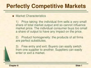
2. The Market Supply Curve • The market supply curve determines the equilibrium price faced by an individual producer. • Equilibrium price – The price at which the quantity of a good demanded in a given time period equals the quantity supplied. • Market supply – The total quantities of a good that sellers are willing and able to sell at alternative prices in a given time period, ceteris paribus.

3. The Market Supply Curve • The market supply curve is the sum of the marginal cost curves of all the firms. • Marginal cost (MC) – The increase in total cost associated with a one-unit increase in production.

4. The Market Supply Curve • Whatever determines marginal cost also determines the competitive firm’s supply response.

5. The Market Supply Curve • The market supply of a competitive industry is determined by: • The price of factor inputs. • Technology. • Expectations. • Taxes. • The number of firms in the industry.

6. Farmer A Farmer B Farmer C Market supply $5 MCA MCB MCC 4 b c d a 3 Price 2 1 0 20 40 60 0 20 40 60 0 20 40 60 0 100 200 Quantity Quantity Quantity Quantity Competitive Market Supply + + =

7. Entry and Exit • Investment decisions shift the market supply curve to the right. • Investment decision - The decision to build, buy, or lease plant and equipment; to enter or exit an industry.

8. Entry and Exit • The profit motive drives these investment decisions. • If there are economic profits, more firms will enter the industry increasing market supply. • Each firm will respond to the resulting lower price and profits by reducing output.

9. Price Quantity Quantity Market Entry Market entry pushes price down and . . . Reduces profits of competitive firm S1 MC S2 ATC E1 f1 p1 p1 f1 p2 p2 E2 Market demand New firms enter q1 q2

10. Tendency Toward Zero Profits • An increase in market supply causes the economic profits to disappear. • Economic profits – The difference between total revenues and total economic costs.

11. Tendency Toward Zero Profits • When economic profits disappear, entry ceases and the market price stabilizes. • Acompetitive market is a market in which no buyer or seller has market power.

12. Tendency Toward Zero Profits • As long as it is easy for existing producers to expand production or for new firms to enter an industry, economic profits will not last long.

13. Low Barriers to Entry • Barriers to entry are obstacles that make it difficult or impossible for would-be producers to enter a particular market.

14. Low Barriers to Entry • Barriers to entry may include: • Patents. • Control of essential factors of production. • Control of distribution outlets. • Well-established brand loyalty. • Government regulation.

15. Market Characteristics of Perfect Competition • Some of the structures, behaviors and outcomes of a competitive market are: • Many firms - none of which has a significant share of total output. • Perfect information - buyers and sellers have complete information on supply, demand, and prices.

16. Market Characteristics of Perfect Competition • Some of the structures, behaviors and outcomes of a competitive market are: • Identical products - products are homogeneous; one firm’s products is the same as any other’s. • MC = p - all competitive firms seek to expand output until marginal cost equals the product’s market price.

17. Market Characteristics of Perfect Competition • Some of the structures, behaviors and outcomes of a competitive market are: • Low barriers to entry - entry barriers are low, economic profits will attract more firms. • Zero economic profit - market supply expands as long as there are economic profits, pushing prices and economic profits down.

18. Competition at Work: Microcomputers • Few, if any, product markets are perfectly competitive. • Many industries function much like a competitive market. • The microcomputer market illustrates how the process of competition works.

19. Market Evolution • As in other industries, the computer industry has evolved over time. • It was never a monopoly, nor was it ever perfect competition.

20. Initial Conditions: The Apple I • Steve Jobs and Steven Wozniak created the Apple Computer Corporation in 1977. • Other companies noted the profits and, due to the low barriers to entry, followed Apple’s lead.

21. The Production Decision • Each competitive firm seeks to make the best short-run production decision. • Production decision - The selection of the short-run rate of output (with existing plant and equipment).

22. The Production Decision • To maximize profit, each competitive firm seeks the rate of output at which marginal cost equals price.

23. The computer industry The typical firm Market equilibrium $1200 1200 Market price C 1000 1000 P = MR Profits 800 800 Market supply Price (per computer) PRICE OR COST Average total cost D 600 600 m 400 400 Market demand 200 200 0 20 40 60 80 0 200 400 600 800 1000 Quantity (thousands) Quantity Initial Equilibrium in the Computer Market

24. Profit Calculations • A profit-maximizing producer seeks to maximize total profit. • This is not necessarily or even very frequently the same thing as maximizing profit per unit.

25. Profit Calculations • Profit per unit is total profit divided by the quantity produced in a given time period.; price minus average total cost. Total profit = profit per unit X quantity sold

26. Computer Revenues, Costs and Profits

27. Computer Revenues, Costs and Profits

28. The Lure of Profits • In competitive markets, economic profits attract new entrants.

29. Low Entry Barriers • Low entry barriers permit new firms to enter competitive markets.

30. A Shift of Market Supply • The entry of new firms shifts the market supply curve to the right. • New entrants will continue to enter as long as there are economic profits in short-run competitive equilibrium. • Short-run equilibrium: p = MC

31. A Shift of Market Supply • As supply increases, price drops toward the minimum of ATC. • In long-run equilibrium, entry and exit cease, and zero economic profit (that is, normal profit) prevails. • Long-run equilibrium: p = MC = minimum ATC

32. A Shift of Market Supply • Once established, long-run equilibrium will continue until market demand shifts or technological improvement reduces the cost of computer production.

33. $1000 $1000 800 800 Profits Price or Cost (per computer) Price (per computer) 0 20,000 0 500 600 Quantity (computers per month) Quantity (computers per month) The Competitive Price and Profit Squeeze An expanded market supply . . . Lowers price and profits for the typical firm MC S1 ATC S2 Old price G New price H m Market demand

34. $1000 $1000 800 800 Price or Cost (per computer) Price (per computer) 0 20,000 0 500 600 Quantity (computers per month) Quantity (computers per month) The Competitive Squeeze Approaching Its Limit The computer industry The typical firm MC ATC S2 S3 Old price J 700 620 New price K Profits m Market demand

35. Short-run equilibrium (p = MC) Long-run equilibrium (p = MC = ATC) MC MC ATC ATC pS pS Price or Cost Price or Cost pL qS qL Quantity Quantity Short- vs. Long-Run Equilibrium

36. Long-Run Rules for Entry and Exit

37. Home Computers vs. Personal Computers • Once long-run equilibrium was reached in the microcomputer market, producers were forced either: • To develop a better product (to increase demand), or • To reduce costs of production.

38. Home Computers vs. Personal Computers • Manufactures of computers did both —separating the market into home computers and personal computers

39. Price Competition in Home Computers • The home computer market confronted the fiercest form of price competition leaving the only option to make an extra buck to push the cost curve down.

40. Price Competition in Home Computers • Costs were pushed down by reducing the number of components and using more powerful computer chips.

41. Further Supply Shifts • With strong competition, often the only way for a firm to improve profitability is to reduce costs. • Cost reductions were accomplished through technological improvements.

42. Further Supply Shifts • Technological improvements are illustrated by a downward shift of the ATC and MC curves.

43. Price (per computer) Quantity (computers per month) Lower Costs Shifts the Supply Curve Downward Old MC New MC New ATC Old ATC N J $700 R 430 600

44. Shutdowns • Once a firm is no longer able to cover variable costs, it should shut down production. • Theshutdown point is the rate of output at which price equals minimum AVC.

45. Exits • Most firms withdrew from the home computer market due to low profits. • The exit rate in 1983-85 matched the entry rate of 1979-82.

46. The Personal Computer Market • Firms initially competed on the basis of product improvements. • Eventually, firms could not sell all the PCs they produced at prevailing prices. • They were forced to cut their prices. • Many shut down.

47. Competitive Process • Competitive market pressures were a driving force in the spectacular growth of the computer industry. • Consumers reaped substantial benefit from competition in computer markets.

48. Allocative Efficiency: The Right Output Mix • The market mechanism works best in competitive markets. • Market mechanism – the use of market prices and sales to signal desired output (or resource allocations).

49. Allocative Efficiency: The Right Output Mix • High profits in a particular industry indicate consumers want a different mix of output. • A competitive market determines the opportunity cost of producing different goods.

50. Allocative Efficiency: The Right Output Mix • The price signal the consumer gets in a competitive market is an accurate reflection of opportunity cost. • Opportunity cost – The most desired goods or services that are forgone in order to obtain something else.