Download
1 / 35
350 likes | 480 Views
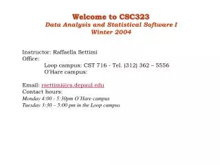
Welcome to CSC323 Data Analysis and Statistical Software I Winter 2004. Instructor: Raffaella Settimi Office: Loop campus: CST 716 - Tel. (312) 362 – 5556 O'Hare campus: Email: rsettimi@cs.depaul.edu Contact hours:

E N D
Welcome to CSC323 Data Analysis and Statistical Software I Winter 2004 Instructor: Raffaella Settimi Office: Loop campus: CST 716 - Tel. (312) 362 – 5556 O'Hare campus: Email: rsettimi@cs.depaul.edu Contact hours: Monday 4:00 - 5:30pm O’Hare campusTuesday 3:30 – 5:00 pm in the Loop campus
Course web page:http://facweb.cs.depaul.edu/rsettimi/323 Check the web page regularly for news and announcements. Course documents and homework assignments will be posted on the course homepage. Lectures can be seen online on the DL website: http://dlweb.cs.depaul.edu The lectures will be available in the morning following the class.
Course topics The course will discuss simple statistical methods and basic concepts of probability theory. The topics of the course are • descriptive statistics and representing data using graphs. • Linear regression models. • Sampling and experimental design. • An introduction to statistical inference • confidence intervals and • hypothesis testing. We will use the statistical package SAS The statistical software SAS runs on • UNIX (accounts on Hawk are available to students) and • on PC's (available in the computer labs) Check the course web page at http://facweb.cs.depaul.edu/rsettimi/323/sasinstructions.htm for more information on SAS availability.
Required Texts: Introduction to the Practice of Statistics, Fourth Edition, by D.S. Moore and G.P. McCabe (2003). ISBN:0-7167-9657-0 Recommended SAS manual SAS Manual for Moore and McCabe's Introduction to the Practice of Statistics. Michael Evans, Freeman. Third edition, 1999. ISBN: 0-7167-3657-8 The course syllabus provides more detailed course information. The syllabus is posted on http://facweb.cs.depaul.edu/rsettimi/323/csc_323.htm
Grading Homework and Programming assignments (35%).No homework this week!! Due on Monday in class or it can be submitted online at http://dlweb.cs.depaul.edu. Late assignments will be accepted not later than three days after the due date (typically by the following Thursday). Notice that a 10% point penalty will be applied for each day after the deadline. Quizzes (15%). There will be two short tests, scheduled tentatively on week 3 and week 8. Students are allowed to bring one single page of notes and a calculator. There will be no make up quizzes. Midterm (30%) on Feb 9th, 2004 at 6:15-7:45pm.It is a closed book exam, students are allowed to bring one single page of notes and a calculator. Final (35%) on March 15th at 6:15 - 8:30 pm. It is a closed book exam, students are allowed to bring two pages of notes and a calculator.
Homework submission • Homework assignments will be posted on Tuesdays. • Homework solutions will be due in class on Monday. (Only legible, organized homework will be graded. Include your name, section number, date, and homework number on the first page of your assignment. Staple pages together.) • Alternatively, homework can be submitted online at the dlweb site http://dlweb.cs.depaul.edu. The online submission application will let you submit only one document, so use a word processor to collate your solutions in a file. • Duplication of homework solutions and computer output prepared in whole or in part by someone else is not permitted.
Lecture 1 Outline • Exploratory data analysis (Sec. 1.1, 1.2) Discovering information from the data through graphs and numbers. • Introduction to the statistical package SAS
Exploratory Data Analysis • The goal of statistics is to gain information from the data. • Data come from several sources: • Available data: • Census data, Federal agencies, Governmental Statistical Offices (www.fedstats.gov), General Social Survey at the University of Chicago’s NORC (http://www.icpsr.umich.edu/GSS/). • Several databases are available on the Internet or at DePaul library!! • New Data: • Sampling from population of interest: Observational studies • Conducting statistical experiments: medical trials, controlled experiments. When well designed, provide most reliable source of information!!
What’s the next step after the data collection? Long listings of data are of little value. Statistical methods come to help us. Exploratory data analysis: set of methods to display and summarize the data. Data on just one variable: the distribution of the observations is analyzed by • Displaying the data in a graph that shows overall patterns and unusual observations (histogram, box plot, density curve) • Computing descriptive statistics that summarize specific aspects of the data (center and spread).
Random variables • Data contain information about group of individuals / subjects • A variable is a characteristic of an observed individual which takes different values for different individuals: • Quantitative variable (continuous) takes numerical values. • Ex.: Height, Weight, Age, Income, Measurements • Qualitative/Categorical variable classifies an individual into categories or groups. • Ex. : Sex, Religion, Occupation, Age (in classes e.g. 10-20, 20-30, 30-40) • The distribution of a variable tells us what values it takes and how often it takes those values • Different statistical methods are used to analyze quantitative or categorical • variables.
Graphs for categorical variables The values of a categorical variable are labels. The distribution of a categorical variable lists the count or percentage of individuals in each category. Counts: 212 168 20 A sample of 400 wireless internet users.
Example: On the morning of April 10, 1912 the Titanic sailed from the port of Southampton (UK) directed to NY. Altogether there were 2,201 passengers and crew members on board. This is the table of the survivors of the famous tragic accident. Define the categorical variables
Bar chart representing the data in the table above (in percentages) Male Female Male Female Survivors Survivors Victims Victims
Graphs for qualitative variables: Stemplots • Stemplot ~ stem-and-leaf plot • To make a stemplot: • Separate each observation into a stem consisting of all but the final (rightmost) digit and a leaf, the final digit. • Write the stems in a vertical column with the smallest at the top, and draw a vertical line at the right of this column. • Write each leaf in the row to the right of its stem, in increasing order out from the stem.
Example: Babe Ruth home run hits 54 59 35 41 46 25 47 60 54 46 49 46 41 34 22 Stem and leaf plot Key 3|5 means35 hits Stems = 1’sLeaves = 1’s 2 5 2 3 5 4 4 1 6 7 6 9 6 1 5 4 9 4 6 0
Stemplots (cont.) • Back-to-back stemplot • How stemplots deal with large data sets? • Splitting stems: • One stem with leaves between 0 and 4 • One stem with leaves between 5 and 9 • How stemplots deal with observations with having many digits? • Rounding
Stemplots (cont.) • Advantages of stemplots: • Describe the shape of a distribution for small numbers • Disadvantages: • Don’t work well with large data sets since they display the values of the variables • Divide the observations into groups (stems) determined by the number system rather than by judgment
Graphs for qualitative variables: the histogram Example: CEO salaries Forbes magazine published data on the best small firms in 1993. These were firms with annual sales of more than five and less than $350 million. Firms were ranked by five-year average return on investment. The data extracted are the age and annual salary of the chief executive officer for the first 60 ranked firms. (Data at http://lib.stat.cmu.edu/DASL/DataArchive.html ) Salary of chief executive officer (including bonuses), in $thousands 145 621 262208 362 424 339 736 29158 498 643 390 332 750 368 659 234 396 300 343 536 543 2172981103 406 254 862 20420625021298 350 800 726 370 536 291 808 543 149 350 242198213296 317 482 155 802 200282 573 388 250 396 572
Drawing a histogram • Construct a distribution table: • Define class intervals or bins (Choose intervals of equal width!) • Count the percentage of observations in each interval • End-point convention: left endpoint of the interval is included, and the right endpoint is excluded, i.e. [a,b[ • Draw the horizontal axis. • Construct the blocks: • Height of block = percentages! • The total area under an histogram must be 100%
30..50% 23.73% 3.39% 1.70% The area of each block represents the percentages of cases in the corresponding class interval (or bin).
Remarks • A histogram represents percent by area. The area of each block represents the percentages of cases in the corresponding class interval. • The total area under a histogram is 100% • There is no fixed choice for the number of classes in a histogram: • If class intervals are too small, the histogram will have spikes; • If class intervals are too large, some information will be missed. • Use your judgment! • Typically statistical software will choose the class intervals for you, but you can modify them.
SMOKING • In a Public Health Service study, a histogram was plotted showing the • number of cigarettes smoked per day by each subject (male current smokers), • as shown below. The density is marked in parentheses. The class intervals • include the left endpoint, but not the right. • The percentage who smoked less than two packs a day but at least a pack, is around (There are 20 cigarettes in a pack.) • 1.5% 15% 30% 50% • The percent who smoked at least a pack a day is around • 1.5% 15% 30% 50% • The percent who smoked at least 3 packs a day is around • 0.25 of 1% 0.5 of 1% 10% • The percent who smoked 20 cigarettes a day is around • 0.35 of 1% 0.5 of 1% 1.5% 3.5% 10%
Answers: • The percentage who smoked less than two packs a day but at least a pack, is around (There are 20 cigarettes in a pack.) • It is given by the area of the third block: 1.5x(40-20)=1.5x20=30% • The percent who smoked at least a pack a day is around • It is given by the area of the third and fourth blocks: 30+0.5x40=50% • The percent who smoked at least 3 packs a day is around • It is the area of the block for number of cigarettes greater or equal to 60. This is half of the fourth block: 10% • The percent who smoked 20 cigarettes a day is around • We use the left endpoint convention, so 20 belongs to the third block. The answer is 1.5%.
Using histograms for comparisons Fuel economy for model year 2001 compact and two-seater cars (Table 1.8 pg 38) City Consumption Highway consumption
Describing distributions with numbers • A distribution can be described through the measures of its center and of its spread. • Measuring the center • The most common measures are the mean or average and the median. • The Mean or Average • To calculate the average of a set of observations, add their value and divide by the number of observations: Data: Number of home runs hit by Babe Ruth as a Yankee 54, 59, 35, 41, 46, 25, 47, 60, 54, 46, 49, 46, 41, 34, 22 The mean number of home runs hit in a year is:
The median • The median M is the midpoint of a distribution, the number such that half the observations are smaller and the other half are larger. • To find the median: • Sort all the observations in order of size from smallest to largest • If the number of observations n is odd, the median M is the center observation in the ordered list; I.e. M=(n+1)/2-th obs. • If the number of observations n is even, the median M is the mean of the two center observations in the ordered list. Example 1: Ordered list of home run hits by Babe Ruth: 22 25 34 35 41 41 46 46 46 47 49 54 54 59 60 N=15 Median = 46 8th Example 2: Ordered list of home run hits by Roger Maris in 1961: 8 13 14 16 23 26 28 33 39 61 N=10 Median = (23+26)/2=24.5
Mean versus Median • The mean and median of a symmetric distribution are close together Symmetric distribution 50% Mean Median • In skewed distributions, the mean is farther out in the long tail than is the median. The mean is more sensitive to extreme values. Left-skewed distribution Right-skewed distribution 50% 50% Mean Median Median Mean
Mean or median? • The mean is a good measure for the center of a symmetric distribution • The median is a resistant measure and should be used for skeweddistributions. Its value is only slightly affected by the presence of extreme observations, no matter how large these observations are.
Example: Shopping in a supermarket A marketing consultant observed 50 consecutive shoppers at a supermarket. The histogram below shows how much each shopper spent in the store. Summary statistics: Mean = $ 34.70 Median = $ 27.855 The mean does not say much… The median says that about 50% of the shoppers spent less than 28 dollars What else would you like to know?
Spread of a Distribution Two measures of spread: 1. The Quartiles: First quartile Q1 = the value such that 25% of the observations fall at or below it, (Q1 is often called 25th percentile). The third quartile Q3 = the value such that 75% of the observations fall at or below it, (Q3 is often called 75th percentile). Typically used if the distribution of the observations is skewed. The Inter-Quartile Range IQR is defined as the distance between the two quartiles: IQR= Q3 – Q1 Q1 M Q3 IQR
Example: Shopping in a supermarket A marketing consultant observed 50 consecutive shoppers at a supermarket. The histogram below shows how much each shopper spent in the store. Summary statistics: Mean = $ 34.70 Median = $ 27.855 Q1 = $19.27 Q3 = $ 45.40 IQR= 45.40-19.27= 26.13 About 50% of the shoppers spent less than 28 dollars, 25% spent less than 20 dollars and 25% of the customers of the store spent more that 45 dollars. Moreover, 50% of the customers spent between 20 and 45 dollars! Extreme values for purchases > Q3 + 1.5xIQR=84.59