Eigen Decomposition and Singular Value Decomposition

1. Eigen Decomposition and Singular Value Decomposition Based on the slides by Mani Thomas Modified and extended by Longin Jan Latecki

2. Introduction Eigenvalue decomposition Spectral decomposition theorem Physical interpretation of eigenvalue/eigenvectors Singular Value Decomposition Importance of SVD Matrix inversion Solution to linear system of equations Solution to a homogeneous system of equations SVD application

3. What are eigenvalues? Given a matrix, A, x is the eigenvector and ? is the corresponding eigenvalue if Ax = ?x A must be square and the determinant of A - ? I must be equal to zero Ax - ?x = 0 ! (A - ?I) x = 0 Trivial solution is if x = 0 The non trivial solution occurs when det(A - ?I) = 0 Are eigenvectors are unique? If x is an eigenvector, then ?x is also an eigenvector and ?? is an eigenvalue A(?x) = ?(Ax) = ?(?x) = ?(?x)

4. Calculating the Eigenvectors/values Expand the det(A - ?I) = 0 for a 2 � 2 matrix For a 2 � 2 matrix, this is a simple quadratic equation with two solutions (maybe complex) This �characteristic equation� can be used to solve for x

5. Eigenvalue example Consider, The corresponding eigenvectors can be computed as For ? = 0, one possible solution is x = (2, -1) For ? = 5, one possible solution is x = (1, 2)

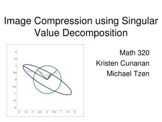
6. Physical interpretation Consider a covariance matrix, A, i.e., A = 1/n S ST for some S Error ellipse with the major axis as the larger eigenvalue and the minor axis as the smaller eigenvalue

7. Physical interpretation Orthogonal directions of greatest variance in data Projections along PC1 (Principal Component) discriminate the data most along any one axis

8. Physical interpretation First principal component is the direction of greatest variability (covariance) in the data Second is the next orthogonal (uncorrelated) direction of greatest variability So first remove all the variability along the first component, and then find the next direction of greatest variability And so on � Thus each eigenvectors provides the directions of data variances in decreasing order of eigenvalues

9. Multivariate Gaussian

10. Bivariate Gaussian

11. Spherical, diagonal, full covariance

12. Let be a square matrix with m linearly independent eigenvectors (a �non-defective� matrix) Theorem: Exists an eigen decomposition (cf. matrix diagonalization theorem) Columns of U are eigenvectors of S Diagonal elements of are eigenvalues of Eigen/diagonal Decomposition

13. Diagonal decomposition: why/how

14. Diagonal decomposition - example

15. Example continued

16. If is a symmetric matrix: Theorem: Exists a (unique) eigen decomposition where Q is orthogonal: Q-1= QT Columns of Q are normalized eigenvectors Columns are orthogonal. (everything is real) Symmetric Eigen Decomposition

17. Spectral Decomposition theorem If A is a symmetric and positive definite k � k matrix (xTAx > 0) with ?i (?i > 0) and ei, i = 1 ? k being the k eigenvector and eigenvalue pairs, then This is also called the eigen decomposition theorem Any symmetric matrix can be reconstructed using its eigenvalues and eigenvectors

18. Example for spectral decomposition Let A be a symmetric, positive definite matrix The eigenvectors for the corresponding eigenvalues are Consequently,

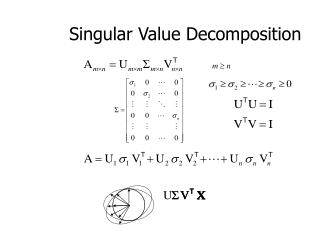
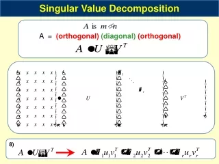
19. Singular Value Decomposition If A is a rectangular m � k matrix of real numbers, then there exists an m � m orthogonal matrix U and a k � k orthogonal matrix V such that ? is an m � k matrix where the (i, j)th entry ?i � 0, i = 1 ? min(m, k) and the other entries are zero The positive constants ?i are the singular values of A If A has rank r, then there exists r positive constants ?1, ?2,??r, r orthogonal m � 1 unit vectors u1,u2,?,ur and r orthogonal k � 1 unit vectors v1,v2,?,vr such that Similar to the spectral decomposition theorem

20. Singular Value Decomposition (contd.) If A is a symmetric and positive definite then SVD = Eigen decomposition EIG(?i) = SVD(?i2) Here AAT has an eigenvalue-eigenvector pair (?i2,ui) Alternatively, the vi are the eigenvectors of ATA with the same non zero eigenvalue ?i2

21. Example for SVD Let A be a symmetric, positive definite matrix U can be computed as V can be computed as

22. Example for SVD Taking ?21=12 and ?22=10, the singular value decomposition of A is Thus the U, V and ? are computed by performing eigen decomposition of AAT and ATA Any matrix has a singular value decomposition but only symmetric, positive definite matrices have an eigen decomposition

23. Applications of SVD in Linear Algebra Inverse of a n � n square matrix, A If A is non-singular, then A-1 = (U?VT)-1= V?-1UT where ?-1=diag(1/?1, 1/?1,?, 1/?n) If A is singular, then A-1 = (U?VT)-1� V?0-1UT where ?0-1=diag(1/?1, 1/?2,?, 1/?i,0,0,?,0) Least squares solutions of a m�n system Ax=b (A is m�n, m�n) =(ATA)x=ATb ) x=(ATA)-1 ATb=A+b If ATA is singular, x=A+b� (V?0-1UT)b where ?0-1 = diag(1/?1, 1/?2,?, 1/?i,0,0,?,0) Condition of a matrix Condition number measures the degree of singularity of A Larger the value of ?1/?n, closer A is to being singular

24. Applications of SVD in Linear Algebra Homogeneous equations, Ax = 0 Minimum-norm solution is x=0 (trivial solution) Impose a constraint, �Constrained� optimization problem Special Case If rank(A)=n-1 (m � n-1, ?n=0) then x=? vn (? is a constant) Genera Case If rank(A)=n-k (m � n-k, ?n-k+1=?= ?n=0) then x=?1vn-k+1+?+?kvn with ?21+?+?2n=1

25. What is the use of SVD? SVD can be used to compute optimal low-rank approximations of arbitrary matrices. Face recognition Represent the face images as eigenfaces and compute distance between the query face image in the principal component space Data mining Latent Semantic Indexing for document extraction Image compression Karhunen Loeve (KL) transform performs the best image compression In MPEG, Discrete Cosine Transform (DCT) has the closest approximation to the KL transform in PSNR

26. Singular Value Decomposition Illustration of SVD dimensions and sparseness

27. SVD example

28. SVD can be used to compute optimal low-rank approximations. Approximation problem: Find Ak of rank k such that Ak and X are both m?n matrices. Typically, want k << r. Low-rank Approximation

29. Solution via SVD Low-rank Approximation

30. Approximation error How good (bad) is this approximation? It�s the best possible, measured by the Frobenius norm of the error: where the ?i are ordered such that ?i ? ?i+1. Suggests why Frobenius error drops as k increased.