Download
1 / 23
240 likes | 272 Views
Learn how to use Pareto Analysis for task prioritization and ABC analysis for inventory management, with emphasis on identifying high priorities, constructing Lorenz curves, and setting reorder points. Understand the 80/20 rule and how to categorize inventory items for efficient control. Follow practical examples to determine reorder points and safety stock levels, ensuring optimal inventory levels and order policies. Enhance your understanding of service levels for different inventory categories and optimize resource allocation.

E N D
Pareto analysis-simplified J.Skorkovský, KPH
What is it ? • tool to specify priorities • which job have to be done earlier than the others • which rejects must be solved firstly • which product gives us the biggest revenues • 80|20 rule
How to construct Lorenz Curve and Pareto chart • list of causes (type of rejects) in % • table where the most frequent cause is always on the left side of the graph
Pareto chart High priorities Lorenz curve
Statements I. • ABC analysis divides an inventory into three categories : • "A items" with very tight control and accurate records • "B items" with less tightly controlled and good records • "C items" with the simplest controls possible and minimal records.
Statements II. • The ABC analysis suggests, that inventories of an organization are not of equal value • The inventory is grouped into three categories (A, B, and C) in order of their estimated importance.
Example of possible allocation into categories • A’ items – 20% of the items accounts for 70% of the annual consumption value of the items. • ‘B’ items - 30% of the items accounts for 25% of the annual consumption value of the items. • ‘C’ items - 50% of the items accounts for 5% of the annual consumption value of the items Beware that 20+30+50=100 and 70+25+5=100 !!
Example of possible categories allocation-graphical representation (4051 items in the stock)
ABC Distribution Minor difference from distribution mentioned before !!
Objective of ABC analysis • Rationalization of ordering policies • Equal treatment OR • Preferential treatment See next slide
Equal treatment 8125 TOTAL INVENTORY (EQT) 1. Value per order= Annual consumption/Numer of orders 2. Average inventory = Value per order/2 see next slide which is taken from EOQ simplified presentation
Resource- Taylor- Wikipedia Carrying cost (will be presented next slide) To verify this relationship, we can specify any number of points values of Q over the entire time period, t , and divide by the number of points. For example, if Q = 5,000, the six points designated from 5,000 to 0, as shown in shown figure, are summed and divided by 6:
Preferential treatment TOTAL INVENTORY (PT) = 4916 8125 TOTAL INVENTORY (EQT)=
Determination of the Reorder Point (ROP) • ROP=expected demand during lead time + safety stock 50-20=30 50=ROP 20
Determination of the Reorder Point (ROP)(home study) • ROP= expected demand during lead time + z* σdLT wherez = numberof standard deviations and σdLT = the standard deviation of lead time demand and z* σdLT=SafetyStock aan
Example(home study) • The manager of a construction supply house determined knows that demand for sand during lead time averages is 50 tons. • The manager knows,that demand during lead time could be described by a normal distribution that has a mean of 50 tons and a standard deviation of 5 tons • The manager is willing to accept a stockout risk of no more than 3 percent
Example-data(home study) • Expectedlead time averages = 50 tons. • σdLT= 5 tons • Risk = 3 % max • Questions : • What value of z(numberof standard deviation)is appropriate? • How much safety stock should be held? • What reorder point should be used?
Example-solution(home study) • Service level =1,00-0,03 (risk)=0,97 and from probability tables you will get z= +1,88 Seenextslidewith probability table
Example-solution(home study) • Service level =1,00-0,03 =0,97 and from probability tables we have got : z= +1,88 • Safety stock = z * σdLT= 1,88 * 5 =9,40 tons • ROP = expected lead time demand + safety stock = 50 + 9.40 = 59.40 tons • For z=1 service level =84,13 % • For z=2 service level= 97,72 % • For z=3 service level = 99,87% (seesix sigma)
ABC and VED and service levels • A items should have low level of service level (0,8 or so ) • B items should have low level of service level (0,95 or so) • C items should have low level of service level (0,95 to 0,98 or so) • D items should have low level of service level (0,8 or so ) • E items should have low level of service level (0,95 or so) • V items should have low level of service level (0,95 to 0,98 or so)
Matrix Resource : https://www.youtube.com/watch?v=tO5MmOBdkxk Prof. Arun Kanda (IIT), 2003