Download
1 / 63
630 likes | 643 Views
Chapter 6: Probability. Probability. Probability is a method for measuring and quantifying the likelihood of obtaining a specific sample from a specific population. We define probability as a fraction or a proportion.

E N D
Probability • Probability is a method for measuring and quantifying the likelihood of obtaining a specific sample from a specific population. • We define probability as a fraction or a proportion. • The probability of any specific outcome is determined by a ratio comparing the frequency of occurrence for that outcome relative to the total number of possible outcomes.
Rolling a die • Event A: even number, greater than 4, or less than 3, etc.
Tossing a coin three times • Event A: one head occurs
a deck of cards • 52 cards: clubs and spades, diamonds and hearts (13 cards in each suit: A, 2, 3, 4, 5, 6, 7, 8, 9, 10, J, Q, K)
Probability (cont'd.) • Whenever the scores in a population are variable, it is impossible to predict with perfect accuracy exactly which score(s) will be obtained when you take a sample from the population. • In this situation, researchers rely on probability to determine the relative likelihood for specific samples. • Thus, although you may not be able to predict exactly which value(s) will be obtained for a sample, it is possible to determine which outcomes have high probability and which have low probability.
Probability and Sampling • To assure that the definition of probability is accurate, the use of random sampling is necessary. • Random samplingrequires that each member of a population has an equal chance of being selected. • Independent random samplingincludes the conditions of random sampling and further requires that the probability of being selected remains constant for each selection
Random Sampling in this textbook(sampling with replacement) • The definition of random sampling in this textbook is similar to “sampling with replacement”, it requires: (1) each individual in the population has an equal chance of being selected. (2) the probability of being selected stays constant from one selection to the next. (~ with replacement)
Random Sampling without Replacement and..... • a random sampling • the probability of being selected changes from one selection to the next... • There are many types of random sampling: e.g. systematic random sampling, stratified random sampling, or cluster sampling....
Random Sampling • for each subject, the probability of being selected = 1/12
With Replacement (independent) independent ↓ • 4 black and 5 red balls dependent
Without Replacement (dependent) • 2 blue and 3 red marbles in the bag
Example 6.1 (p. 168) • N=10, X=1,1,2,3,3,4,4,4,5,6 • random sample, n=1 • P(X>4) = ? • P(X <5) = ?
ex. 1-3 (p. 169) • 1. 19 females, 8 males, 4/19 males and 3/8 females have no siblings • 2. 10 red, 30 blue marbles in a jar (random sampling = with replacement!!) • 3. N=10, n=1,Fig 6.2(p. 168)
Probability (cont'd.) • When a population of scores is represented by a frequency distribution, probabilities can be defined by proportions of the distribution. • Probability values are expressed by a fraction or proportion. • In graphs, probability can be defined as a proportion of area under the curve.
Fig 6.4 (p. 171) check z table (col. D) For z=1.00, the table’s value is 0.3413; times 2 is 0.6826. For z=2.00, the table’s value is 0.4772; times 2 is 0.9544. For z=3.00, the table’s value is 0.4987; times 2 is 0.9974.
Probability and the Normal Distribution • If a vertical line is drawn through a normal distribution, several things occur. • The line divides the distribution into two sections. The larger section is called the body and the smaller section is called the tail. • The exact location of the line can be specified by a z-score.
Normal Distribution • body v.s. tail μ = 500
example 6.2 (p. 171-172) • SAT scores, μ=500, σ=100 • P(X>700) = ? 1st : X=700 z=(700-500)/100=2 2nd : P(z>2) = 0.5-0.4772 = 2.28%
Probability and the Normal Distribution (cont'd.) • The unit normal table lists several different proportions corresponding to each z-score location. (p. 699 - 702) • Column A of the table lists z-score values. • For each z-score location, columns B and C list the proportions in the body and tail, respectively. • Finally, column D lists the proportion between the mean and the z-score location. • Because probability is equivalent to proportion, the table values can also be used to determine probabilities.
Probability and the Normal Distribution (cont'd.) • To find the probability corresponding to a particular score (X value), you first transform the score into a z-score, then look up the z-score in the table and read across the row to find the appropriate proportion/probability. • To find the score (X value) corresponding to a particular proportion, you first look up the proportion in the table, read across the row to find the corresponding z-score, and then transform the z-score into an X value.
Probability and the Normal Distribution (cont'd.) • The normal distribution is symmetrical; therefore, the proportions will be the same for the positive and negative values of a specific z-score. • Proportions are always positive, even if the corresponding z-score is negative. • A negative z-score means that the tail of the distribution is on the left side and the body is on the right, and vice versa for a positive z-score.
example 6.3A (p. 175) • P(z > 1) = ? Fig. 6.8 (a) check z table (p. 700) col. C: P(z < -1) = 0.1587 check col. D: P(z < -1) = 0.5 – P(0<z<1) = 0.5 – 0.3413 = 0.1587
example 6.3B (p. 175) • P( z < 1.5) = ? Fig. 6.8 (b) check col. D in z table P(z < 1.5) = 0.5 + P(0<z<1.5) = 0.5+0.4332 = 0.9332 check z table (p. 701) col. B = P(z < 1.5)=0.9332 or check col. C = P(z < - 1.5) = P(z > 1.5)=0.0668 P(z < 1.5) = 1 – 0.0668 = 0.9332
example 6.3C (p. 175-176) • P(z < -0.5) = ? Fig. 6.8 (c) check z table (p. 700) check col. D in z table P(z < -0.5) = 0.5 – P(0<z<0.5) = 0.5 – 0.1915 = 0.3085 col. C = P(z < -0.5) = 0.3085
example 6.4A (p. 176) • P( z > z0) = 0.1, z0 = ? Fig 6.9 (a) check col. D in z table P(z > ?) =0.5 – P(0<z<?)= 0.1 P(0<z<?)= 0.4 find P(0<z<1.28)= 0.3997 check col. C of p.700 (probability = 0.1003) z0 = 1.28
example 6.4B (p. 176) • P( |z| < z0) = 0.6, z0 = ? Fig 6.9 (b) check col. D of p.700 (probability = 0.2995) P(-? < z < ?) =0.6P(0 < z < ?)= 0.3 find P(0<z<0.84)= 0.2995 z0 = 0.84
ex. 2(p. 177) • P( z > z0) = 0.2, z0 = ? check col. D in z table P(z > ?) =0.5 – P(0<z<?)= 0.2 P(0<z<?)= 0.3 find P(0<z<0.84)= 0.2995 check col. C of p.700 (probability = 0.2005) • z0 = 0.84 b. P( z > z0) = 0.6, z0 = ? check col. D in z table P(z > ?) =0.5 – P(0<z<?)= 0.6 P(0<z<?)= 0.1 find P(0<z<0.25)= 0.0987z0 = -0.25 check col. B of p.699 (probability = 0.5987) • z0 = -0.25 c. P( |z| < z0) = 0.7, z0 = ? check col. D in z table 2*P(0<z < ?) =0.7P(0<z<?)= 0.35 find P(0<z<1.04)= 0.3508z0 = 1.04 check col. D of p.700 (probability = 0.3508) z0 = 1.04
6.3 From X to z (p.178) • If X is normally distributed, then you can use z score and z distribution to find the probability. • If X is not from a normal distribution, you should not just assume it’s normal and use z table to find the probability for X.
example 6.5 (p. 178) • IQ scores ~ Normal, μ = 100, σ=15 • P(X < 120) = ? • z = (120-100)/15 = 1.33 • P(z < 1.33) = ? • check D P(z < 1.33) = 0.5+P(0<z<1.33) = 0.5+0.4082 = 0.9082 • The probability of randomly selecting a person with IQ less than 120 is 0.9082. • The proportion of the individuals in the population with IQ less than 120 is 0.9082.
Percentiles and Percentile Ranks • The percentile rank for a specific X value is the percentage (%) of individuals with scores at or below that value. • When a score is referred to by its rank, the score X is called a percentile. The percentile rank for a score in a normal distribution is simply the proportion to the left of the score. • in ex. 6.5: the percentile rank for IQ = 120 is 0.9082
example 6.6 (p. 179) • (interstate highway) driving speed X miles/hour • μ = 58, σ=10 (it is approximately normal) • P(55 < X < 65) = ? • P( –0.3 < z < 0.7) = P(z > -0.3) – P(z > 0.7) check col. B, C • =0.6179 – 0.2420 = 0.3759 or check col. D P( – 0.3 < z < 0.7) = P( 0< z < 0.3) + P( 0< z < 0.7) = 0.1179+0.2580 = 0.3759
example 6.7 (p. 180) • (interstate highway) driving speed X miles/hour • μ = 58, σ=10 (approximately normal) • P(65 < X < 75) = ? • P( 0.7 < z < 1.7) = P(z > 0.7) – P(z > 1.7) check col. C • =0.2420 – 0.0446 = 0.1974 or check col. D P( 0.7 < z < 1.7) = P( 0< z < 1.7) – P( 0< z < 0.7) = 0.4554+0.2580 = 0.1974
example 6.8 (p. 182) • time commuting to work: minutes/day • μ = 24.3, σ=10 (assumed normal) • P( X > X0) = 0.1, X0=? • P(z > z0) = 0.1, z0 = ? check col. D in z table P(z > ?) =0.5 – P(0<z<?)= 0.1 P(0<z<?)= 0.4 find P(0<z<1.28)= 0.3997 • z0 =1.28 X0= 1.28*10 + 24.3 = 37.1 10% of people spend more than 37.1 minutes of commuting time each day
example 6.9 (p. 183) • time commuting to work: minutes/day • μ = 24.3, σ=10 (assumed normal) • P( |X| < X0) = P( |z| < z0) = 0.9, X0 = ? • check col. D for 45% P(0 < z < ?) = 0.45 • P(0 < z < 1.64) = 0.4495, P(0 < z < 1.65) = 0.4505 • z0 =1.645 X0 = 1.645*10 + 24.3 = 40.75 • z0 =-1.645 X0 = -1.645*10 + 24.3 = 7.85 90% of people spend between 7.85 and 40.75 minutes of commuting time each day
ex. 2 (p. 184) • SAT(math): μ = 500, σ=100 (assumed normal) • a. P( X > X0) = 0.6, minimum score: X0 =? • P(z > ?) =0.5 + P(0<z<?)= 0.6 P(0<z<?)= 0.1 • P(0 < z < 0.25) = 0.0987 = P( -0.25 < z < 0) • X0 = (-0.25)*100+500 = 475 • b. P( X > X0) = 0.1, minimum score: X0 =? • P(z > ?) =0.5 – P(0<z<?)= 0.1 P(0<z<?)= 0.4 • P(0 < z < 1.28) = 0.3997 • X0 = 1.28*100+500 = 628 • c. P( |X| < X0) = P( |z| < z0) = 0.5, X0 = ? • P( – ? < z < ?) = 2*P( 0< z < ?) = 0.5 P( 0< z < ?) = 0.25 • P(0 < z < 0.67) = 0.2486X0 = 0.67*100+500 = 567, • X0 = – 0.67*100+500 = 433
ex. 3 (p. 184) • positively skewed, μ = 40, σ=10 • find P(X > 45) = ? lack the info about the degree of skewness impossible to find P(X > 45)
Probability and the Binomial Distribution • Binomial distributions are formed by a series of observations (for example, 100 coin tosses) for which there are exactly two possible outcomes (heads and tails) • The two outcomes are identified as A and B, with probabilities of p(A) = p and p(B) = q. • p + q = 1.00 • The distribution shows the probability for each value ofX, where X is the number of occurrences of A in a series of n observations.
Probability and the Binomial Distribution (cont.) • The outcome of each trial is classified into one of two mutually exclusive categories—a successor a failure • The random variable, x, is the number of successes in a fixed number of trials (n). • Theprobability of success and failure stay the same for each trial. P(success) = P(A) = p • Thetrials are independent, meaning that the outcome of one trial does not affect the outcome of any other trial. (with replacement)
example 6.10 (p. 185-186) • toss a fair coin twice • X: # of heads • HH, HT, TH, TT • each has probability = ¼ • P(X=0)=P(X=2)=¼ • P(X=1)=½ • P(X≥1)=P(X=1)+P(X=2)=¾ binomial distribution is a discrete probability distribution.
Probability after n Coin tosses p.186 x : number of heads after tossing a fair coin n times
Binomial – Shapes or Skewness for Varying and n = 10, = 0.5(symmetric) The shape of a binomial distribution changes as n and change. Here we haven = 10
Binomial – Shapes or Skewness for Constant and Varying n: = 0.1,n larger more symmetric