Download
1 / 62
650 likes | 1.04k Views
Chapter 4: Probability. Limiting Relative Frequency. Chapter Goals. Learn the basic concepts of probability. Learn the rules that apply to the probability of both simple and compound events.

E N D
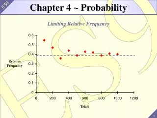
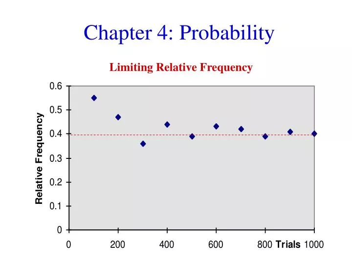
Chapter 4: Probability Limiting Relative Frequency
Chapter Goals • Learn the basic concepts of probability. • Learn the rules that apply to the probability of both simple and compound events. • In order to make inferences, we need to study sample results in situations in which the population is known.
4.1: The Nature of Probability Example: Consider an experiment in which we roll two six-sided fair dice and record the number of threes face up. The only possible outcomes are 0 three’s, 1 three, or 2 three’s. Here are the results after 100 and after 1000 rolls.
We can express these results (from the 1000 rolls) in terms of relative frequencies and display the results using a histogram.
If we continue this experiment for several thousand more rolls: 1. The frequencies will have approximately a 25:10:1 ratio in totals. 2. The relative frequencies will settle down. Note: We can simulate many probability experiments. 1. Use random number tables. 2. Use a computer to randomly generate number values representing the various experimental outcomes. 3. Key to either method is to maintain the probabilities.
4.2: Probability of Events Probability that an Event Will Occur: The relative frequency with which that event can be expected to occur. The probability of an event may be obtained in three different ways: Empirically Theoretically Subjectively
Experimental or empirical probability: 1. The observed relative frequency with which an event occurs. 2. Prime notation is used to denote empirical probabilities: 3. n(A): number of times the event A has occurred. 4. n: number of times the experiment is attempted. Question: What happens to the observed relative frequency as n increases?
Example: Consider tossing a fair coin. Define the event H as the occurrence of a head. What is the probability of the event H, P(H)? 1. In a single toss of the coin, there are two possible outcomes. 2. Since the coin is fair, each outcome (side) should have an equally likely chance of occurring. 3. Intuitively, P(H) = 1/2 (the expected relative frequency). Note: (a) This does not mean exactly one head will occur in every two tosses of the coin. (b) In the long run, the proportion of times that a head will occur is approximately 1/2.
To illustrate the long-run behavior: 1. Consider an experiment in which we toss the coin several times and record the number of heads. 2. A trial is a set of 10 tosses. 3. Graph the relative frequency and cumulative relative frequency of occurrence of a head. 4. A cumulative graph demonstrates the idea of long-run behavior. 5. This cumulative graph suggests a stabilizing, or settling down, effect on the observed cumulative probability. 6. This stabilizing effect, or long-term average value, is often referred to as the law of large numbers.
Relative Frequency: Expected value = 1/2 Trial
Expected value = 1/2 Cumulative Relative Frequency:
Law of Large Numbers: If the number of times an experiment is repeated is increased, the ratio of the number of successful occurrences to the number of trials will tend to approach the theoretical probability of the outcome for an individual trial. Interpretation: The law of large numbers says: the larger the number of experimental trials n, the closer the empirical probability (A) is expected to be to the true probability P(A). In symbols: As
4.3: Simple Sample Spaces • We need to talk about data collection and experimentation more precisely. • With many activities, like tossing a coin, rolling a die, selecting a card, there is uncertainty as to what will happen. • We will study and characterize this uncertainty.
Experiment: Any process that yields a result or an observation. Outcome: A particular result of an experiment. Example: Suppose we select two students at random and ask each if they have a car on campus. 1. A list of possible outcomes: (Y, Y), (Y, N), (N, Y), (N, N) 2. This is called ordered pair notation. 3. The outcomes may be displayed using a tree diagram.
Tree diagram: Student 1 Student 2 Outcomes Y Y, Y Y N Y, N Y N, Y N N N, N 1. This diagram consists of four branches: 2 first generation branches and 4 second generation branches. 2. Each branch shows a possible outcome.
Sample Space: The set of all possible outcomes of an experiment. The sample space is typically called S and may take any number of forms: a list, a tree diagram, a lattice grid system, etc. The individual outcomes in a sample space are called sample points. n(S) is the number of sample points in the sample space. Event: any subset of the sample space. If A is an event, then n(A) is the number of sample points that belong to A. Example: For the student car example above: S = { (Y, Y), (Y, N), (N, Y), (N, N) } n(S) = 4
Example: An experiment consists of two trials. The first is tossing a penny and observing a head or a tail; the second is rolling a die and observing a 1, 2, 3, 4, 5, or 6. Construct the sample space. S = { H1, H2, H3, H4, H5, H6, T1, T2, T3, T4, T5, T6 } Example: Three voters are randomly selected and asked if they favor an increase in property taxes for road construction in the county. Construct the sample space. S = { NNN, NNY, NYN, NYY, YNN, YNY, YYN, YYY}
Example: An experiment consists of selecting electronic parts from an assembly line and testing each to see if it passes inspection (P) or fails (F). The experiment terminates as soon as one acceptable part is found or after three parts are tested. Construct the sample space. Outcome F FFF F F P FFP P FP P P S = { FFF, FFP, FP, P }
Example: The 1200 students at a local university have been cross tabulated according to resident and college status: The experiment consists of selecting one student at random from the entire student body. n(S) = 1200
Example: On the way to work, some employees at a certain company stop for a bagel and/or a cup of coffee. The accompanying Venn diagram summarizes the behavior of the employees for a randomly selected work day. The experiment consists of selecting one employee at random. n(S) = 77 Coffee Bagel
Note: 1. The outcomes in a sample space can never overlap. 2. All possible outcomes must be represented. 3. These two characteristics are called mutually exclusive and all inclusive.
4.4: Rules of Probability • Consider the concept of probability and relate it to the sample space. • Recall: the probability of an event is the relative frequency with which the event could be expected to occur, the long-term average.
Equally Likely Events: 1. In a sample space, suppose all sample points are equally likely to occur. 2. The probability of an event A is the ratio of the number of sample points in A to the number of sample points in S. 3. In symbols: 4. This formula gives a theoretical probability value of event A’s occurrence. 5. The use of this formula requires the existence of a sample space in which each outcome is equally likely.
Example: A fair coin is tossed 5 times, and a head (H) or a tail (T) is recorded each time. What is the probability of A = {exactly one head in 5 tosses}, and B = {exactly 5 heads}? The outcomes consist of a sequence of 5 H’s and T’s A typical outcome: HHTTH There are 32 possible outcomes, all equally likely. A = {HTTTT, THTTT, TTHTT, TTTHT, TTTTH} B = {HHHHH}
Subjective Probability: 1. Suppose the sample space elements are not equally likely, and empirical probabilities cannot be used. 2. Only method available for assigning probabilities may be personal judgment. 3. These probability assignments are called subjective probabilities. 4. Personal judgment of the probability is expressed by comparing the likelihood among the various outcomes.
Basic Probability Ideas: 1. Probability represents a relative frequency. 2. P(A) is the ratio of the number of times an event can be expected to occur divided by the number of trials. 3. The numerator of the probability ratio must be a positive number or zero. 4. The denominator of the probability ratio must be a positive number (greater than zero). 5. The number of times an event can be expected to occur in n trials is always less than or equal to the total number of trials, n.
Properties: 1. The probability of any event A is between 0 and 1. 2. The sum of the probabilities of all outcomes in the sample space is 1. Note: 1. The probability is zero if the event cannot occur. 2. The probability is one if the event occurs every time (a sure thing).
Example: On the way to work Bob’s personal judgment is that he is four times more likely to get caught in a traffic jam (TJ) than have an easy commute (EC). What values should be assigned to P(TJ) and P(EC)?
Odds: another way of expressing probabilities. If the odds in favor of an event A are a to b, then 1. The odds against A are b to a. 2. The probability of event A is 3. The probability that event A will not occur is
Example: The odds in favor of you passing an introductory statistics class are 11 to 3. Find the probability you will pass and the probability you will fail. Using the preceding notation: a = 11 and b = 3. Complement of an Event: The set of all sample points in the sample space that do not belong to event A. The complement of event A is denoted by (read “A complement”).
Example: 1. The complement of the event “success” is “failure.” 2. The complement of the event “rain” is “no rain.” 3. The complement of the event “at least 3 patients recover” out of 5 patients is “2 or fewer recover.” Note: 1. 2. 3. Every event A has a complementary event 4. Complementary probabilities are very useful when the question asks for the probability of “at least one.”
Example: A fair coin is tossed 5 times, and a head(H) or a tail (T) is recorded each time. What is the probability of A = {at least one head in 5 tosses}, B = {at most 3 heads in 5 tosses}?
Example: A local automobile dealer classifies purchases by number of doors and transmission type. The table below gives the number of each classification. If one customer is selected at random, find the probability that 1. The selected individual purchased a car with automatic transmission. 2. The selected individual purchased a 2-door car.
4.5: Mutually Exclusive Events and the Addition Rule • Compound Events: formed by combining several simple events. • The probability that either event A or event B will occur: P(A or B). • The probability that both events A and B will occur: P(A and B). • The probability that event A will occur given that event B has occurred: P(A | B)
Mutually Exclusive Events: Events defined in such a way that the occurrence of one event precludes the occurrence of any of the other events. (In short, if one of them happens, the others cannot happen.) Note: 1. Complementary events are also mutually exclusive. 2. Mutually exclusive events are not necessarily complementary.
Example: The following table summarizes visitors to a local amusement park. One visitor from this group is selected at random. 1. Define the event A as “the visitor purchased an all-day pass.” 2. Define the event B as “the visitor selected purchased a half-day pass.” 3. Define the event C as “the visitor selected is female.”
Solution: 1. The events A and B are mutually exclusive. 2. The events A and C are not mutually exclusive. The intersection of A and C can be seen in the table above or in the Venn diagram below.
General Addition Rule: Let A and B be two events defined in a sample space S. Illustration: Note: If two events A and B are mutually exclusive:
Special Addition Rule: Let A and B be two events defined in a sample space. If A and B are mutually exclusive events, then This can be expanded to consider more than two mutually exclusive events:
Example: All employees at a certain company are classified as only one of the following: manager (A), service (B), sales (C), or staff (D). It is known that P(A) = .15, P(B) = .40, P(C) = .25, and P(D) = .20
Example: A consumer is selected at random. The probability the consumer has tried a snack food (F) is .5, tried a new soft drink (D) is .6, and tried both the snack food and the soft drink is .2.
4.6: Independence, the Multiplication Rule, and Conditional Probability Independent Events: Two events A and B are independent events if the occurrence (or nonoccurrence) of one does not affect the probability assigned to the occurrence of the other. Note: If two events are not independent, they are dependent.
Background: 1. Sometimes two events are related in such a way that the probability of one depends upon whether the second event has occurred. 2. Partial information may be relevant to the probability assignment. Conditional Probability: The symbol P(A | B) represents the probability that A will occur given B has occurred. This is called conditional probability. 1. 2. Given B has occurred, the relevant sample space is no longer S, but B (reduced sample space). 3. A has occurred if and only if the event A and B has occurred.
Independent Events: Two events A and B are independent events if P(A | B) = P(A) or P(B | A) = P(B) Note: 1. If A and B are independent, the occurrence of B does not affect the occurrence of A. 2. If A and B are independent, then so are: 3. Independence cannot be shown on a Venn diagram.
Example: Consider the experiment in which a single fair die is rolled: S = {1, 2, 3, 4, 5, 6 }. Define the following events: A = “a 1 occurs,” B = “an odd number occurs,” and C = “an even number occurs.”
Example: In a sample of 1200 residents, each person was asked if he or she favored building a new town playground. The responses are summarized in the table below. If one resident is selected at random, what is the probability the resident will: 1. Favor the new playground? 2. Favor the playground if the person selected is less than 30? 3. Favor the playground if the person selected is more than 50? 4. Are the events F and M independent?
General Multiplication Rule: Let A and B be two events defined in sample space S. Then or Note: How to recognize situations that result in the compound event “and.” 1. A followed by B. 2. A and B occurred simultaneously. 3. The intersection of A and B. 4. Both A and B. 5. A but not B (equivalent to A and not B).