Download
1 / 28
280 likes | 283 Views
Synchronic Magnetic Maps - the Inner Boundary Condition for the Heliosphere. David Hathaway NASA Marshall Space Flight Center 2011 August 2 – Space Weather Summer School http://solarscience.msfc.nasa.gov/presentations.html. The Sun’s Global Magnetic Field.

E N D
Synchronic Magnetic Maps - the Inner Boundary Condition for the Heliosphere David Hathaway NASA Marshall Space Flight Center 2011 August 2 – Space Weather Summer School http://solarscience.msfc.nasa.gov/presentations.html
The Sun’s GlobalMagnetic Field The photospheric magnetic field is the inner boundary condition for virtually all space weather applications and predictions. The photospheric field extends into the corona and the solar wind and provides the context for CME, SEP, and GCR propagation. Extrapolations of the photospheric field require the field to be specified over the entire surface – including both poles and the backside.
Field Extrapolations The magnetic field measured in the photosphere is used in field extrapolations to determine the magnetic structures associated with solar eruptions. Prominence eruption from Yeates, Mackay, & van Ballegooijen (2008).
Field Extrapolations The magnetic field measured in the photosphere is used in field extrapolations to determine the structure and dynamics of the corona and the solar wind. Open field and high speed solar wind from Wang, Robbrecht, & Sheeley (2009).
Synoptic Map Construction • One map from each rotation of the Sun using data from near the central meridian. They do show: • 1) Bi-polar active regions are the primary sources for the field • 2) Diffusion (random walk in longitude and latitude) • 3) Differential Rotation (faster at the equator, slower near the poles) • 4) Meridional Flow (poleward from the equator )
Synoptic Map Data at Carrington longitude 0 is adjacent to data at Carrington longitude 360 but are acquired 27 days later. Much has changed!
The Goal: Produce instantaneous (synchronic) magnetic maps of the entire surface of the Sun. The Problem: We only see one hemisphere at any time and that view excludes each pole for six months of each year. A Near Term Solution: Model the transport of magnetic field at the surface of the Sun using Earthside and farside information. A Long-Term Solution: Four or five spacecraft with magnetographs: one near Earth, one in the ecliptic 120° ahead of Earth, one in the ecliptic 120° behind Earth, and at least one more - out of the ecliptic where it can observe the other pole.
Synchronic Map Construction • Data assimilation • Magnetic data from full disk • Active region data from farside helioseismology • Active region data from active region decay • Flux transport • Differential rotation structure and variations • Meridional flow structure and variations • Supergranule diffusion (random walk) model
Surface Flux Transport • Surface magnetic flux transport models were developed in the early 1980s by the Naval Research Laboratory (NRL) group including Neil Sheeley, Yi-Ming Wang, Rick DeVore, and Jay Boris. They found that they could reproduce the evolution of the Sun’s surface magnetic field using active region flux emergence as the only source of magnetic flux – that flux is then transported across the Sun’s surface by: • Differential Rotation, U(θ) • Meridional Flow, V(θ) • Supergranule Diffusion, • ∂B/∂t + 1/(R sinθ) ∂(BV sinθ)/∂θ + 1/(R sinθ) ∂(BU)/∂ = 2B + S(θ,) • Neither the meridional flow nor the supergranule diffusion were well constrained at that time – so they used what worked.
Characterizing the Axisymmetric Flows We (Hathaway & Rightmire 2010, Science, 327, 1350) measured the axisymmetric transport of magnetic flux by cross-correlating 11x600 pixel strips at 860 latitude positions between ±75˚ from magnetic images acquired at 96-minute intervals by MDI on SOHO.
Average Flow Profiles Our MDI data included corrections for CCD misalignment, image offset, and a 150 year old error in the inclination of the ecliptic to the Sun’s equator. We extracted differential rotation and meridional flow profiles from over 60,000 image pairs from May of 1996 to September of 2010. Average (1996-2010) differential rotation profile with 2σ error limits. Average (1996-2010) meridional flow profile with 2σ error limits.
Meridional Flow Comparisons The Meridional Flow we measure is very unlike that still used by the NRL group (Wang et al.). It is similar at low latitudes to that used by other groups but differs by not vanishing at high latitudes.
Solar Cycle Variations in the Axisymmetric Flows While the differential rotation does vary slightly over the solar cycle, it is the meridional flow that shows the most significant variation. The Meridional Flow slowed from 1996 to 2001 but then increased in speed again after maximum. The slowing of the meridional flow at maximum seems to be a regular solar cycle occurrence (Komm, Howard, & Harvey, 1993). The greater speed up after maximum is specific to Cycle 23. Differential rotation variations Meridional flow variations
Solar Cycle Variations in Flow Structure The differential rotation and meridional flow profiles for each solar rotation also show that the differential rotation changes very little while the meridional flow changes substantially. Note, in particular, the presence of countercells with equatorward flow near the poles. Differential rotation profiles Meridional flow profiles
Complications The axisymmetric flows we (Hathaway & Rightmire 2010, 2011) measured were for magnetic elements with |B| < 500G. Lisa has discovered that if she limits the data to weaker magnetic elements she finds faster meridional flow and slower differential rotation. The weaker magnetic elements are anchored closer to the surface shear layer where the rotation is slower and meridional flow faster. This makes magnetic flux transport more complicated!
Supergranules and the Magnetic Network Tracking the motions of granules (correlation tracking with 6-minute time lags from HMI Intensity data) reveals the flow pattern within supergranules and the relationship with the magnetic pattern – the magnetic network forms at the supergranule boundaries (convergence zones).
Flux Transport Details Four days of HMI data drive home the fact that flux transport is dominated by the cellular flows. The extent to which this can be represented by a diffusion coefficient and a Laplacian operator is to be determined. 300 Mm 500 Mm
Characterizing Supergranules We (Hathaway et al. 2010, ApJ 725, 1082) analyzed and simulated Doppler velocity data from MDI to determine the characteristics of supergranulation. These cellular flows have a broad spectrum characterized by a peak in power at wavelengths of about 35 Mm. MDI SIM
Measuring their motions The axisymmetric flows can be measured using the Doppler velocity pattern using the same method used with the magnetic pattern. A key difference is the use of several different time lags between images.
Reproducing the Lifetimes The cellular structures are given finite lifetimes by adding random perturbations to the phases of the complex spectral coefficients. The amplitude of the perturbation was inversely proportional to a lifetime given by the size of the cell (from its wavenumber) divided by its flow velocity (from the amplitude of the spectral coefficient). This process can largely reproduce the strength of the cross-correlation as a function of both time and latitude.
Supergranule Diffusion We can use the evolving supergranule flow field from the simulation to transport magnetic elements from an initial magnetic map and use this to determine the diffusion coefficient, . (Lisa Rightmire)
Reproducing their Rotation The motions of the cellular patterns in longitude can be reproduced by making systematic changes to the complex spectral coefficient phases (Hathaway et al. 2010).
Reproducing their Meridional Flow The motions of the cellular patterns in latitude can be reproduced by making systematic changes to the complex spectral coefficient amplitudes (Hathaway et al. 2010).
Supergranules Rule! Surprisingly, if we add differential rotation and meridional flow on top of supergranules that don’t move with those flows we get magnetic element motion with no differential rotation or meridional flow. The differential rotation and meridional flow velocities are too small to overpower the flows in the supergranules themselves!
Supergranules Rule! The magnetic elements experience differential rotation and meridional flow only to the extent that supergranules are transported by these flows - as in this simulation.
Data Assimilation Data from the entire visible hemisphere should be assimilated – but with weights inversely proportional to the noise level. Knowledge of the growth and decay of active regions can allow for estimates of active region evolution after they rotate off of the west limb. Farside imaging from helioseismology can provide information about the emergence of new active regions on the farside of the Sun.
Synchronic Map Examples Full disk data assimilated with weights that vary inversely with noise and decay exponentially with time. Flux is transport by differential rotation by taking the FFT in longitude of the data (and weights) at each latitude and adding a phase shift representing the longitudinal displacement. Updated 15 times per day
Conclusions To produce synchronic magnetic maps for heliospheric conditions we need to transport magnetic flux and assimilate data from multiple sources. To do the axisymmetric transport we need to measure and monitor the structure and variations in the flow components – differential rotation and meridional flow. To do the non-axisymmetric transport (diffusion) we need to characterize the supergranule flow properties. Magnetic elements experience differential rotation and meridional flow via the differential rotation and meridional motion of supergranules.