Download
1 / 21
310 likes | 514 Views
Chapter 11: Probability. Objectives. Define probability Work with mutually exclusive events Work with independent events Work with dependent events Calculate expected monetary values Recognise and calculate binomial probabilities. Defining Probability. Most commonly used definition:.

E N D
Objectives • Define probability • Work with mutually exclusive events • Work with independent events • Work with dependent events • Calculate expected monetary values • Recognise and calculate binomial probabilities
Defining Probability Most commonly used definition: Number of ways event can occur Number of outcomes P(Event) = For example, a coin has 2 sides, so probability of a Head is 1/2 The problem is that not all outcomes are necessarily equally likely or equally probable (Think of a biased dice) BUT
More Definitions Frequency definition: Number of times event occurs Number of trials P(Event) = Subjective definition: Ask a series of “experts” to estimate the probability and use feedback to refine the figure Axiomatic approach: Set up axioms and derive probability results from these
Mutually Exclusive Events If two (or more) events cannot happen at the same time, they are called mutually exclusive. This could be different scores on a die, since only one face can show at a time. In this case we can just add the probabilities together: P(1) + P(2) = 1/6 + 1/6 = 1/3 = P(1 or 2) Rule 1: Where A and B are mutually exclusive, then: P(A or B) = P(A) + P(B)
Non-Mutually Exclusive Events Some items or events have more than one characteristic If you think of a pack of cards, each card has a value and a suit. Sample space: Rule 2: Where A and B are not mutually exclusive, then: P(A or B) = P(A) + P(B) – P(A and B)
Independent Events If the outcome of one event does not affect the outcome of some other event, then the 2 events are independent For example, if two coins are tossed, the result on the first coin has no effect on the result on the second coin So we can multiply the probabilities P(H on 1st) x P(H on 2nd) = ½ x ½=¼ = P(H on both coins) Rule 3 Where A and B are independent, then: P(A & B) = P(A) x P(B)
Dependent Events Where the outcome of one event affects the outcome of a second event, the second event is called dependent For example, if we have a small group of people consisting of 3 men and 4 women and want to find probabilities relating to selecting 2 people, then the probability relating to the second person will depend on who was selected first. First Person P(Man) = 3/7 P(Woman) = 4/7 2nd person if 1st Male P(Man) = 2/6 P(Woman) = 4/7 2nd person if 1st Female P(Man) = 3/6 P(Woman) = 3/7
Expected Values Probability is a useful concept, but many people find it a little difficult, unless they are doing a course such as this. They will want to know what the effect or outcome is, and we can help by talking about what is expected to happen This expectation is a sort of “average in the long run” And we find it by multiplying the effect by the probability So, if we have a lottery ticket which might win £1,000 with a probability of 0.001, but win nothing otherwise, then we have the expected value of the ticket as: £1,000x0.001 + £0x0.999 = £1 Don’t think this is what will happen – it can’t! It is the average value of the ticket, so don’t pay £2 for it!
Decision Trees This is a way of illustrating the consequences of decisions and the outcomes of events for which we can assign probabilities As a visual medium, it can help communicate ideas to other people It can also help you to think through a problem, making sure that you have considered every option. When using decision trees we are usually dealing with monetary outcomes, so rather than expected values, we usually talk about Expected Monetary Values
Decision Trees (2) Think about the following example: A company is deciding whether or not to expand. If they expand, at a cost of £50,000 and the market also expands, their expected increase in profit is £100,000 per year. Expansion without an increase in the market might give increased profits of £20,000 per year. If they do not expand and the market grows, they will still increase their profits by £20,000 per year, but if the market does not grow, then there is no foreseeable increase in profits. The probability the market grows as predicted is 0.25
Decision Trees (3) For the expand company option, we have: Expected Profit Market expands p=0.25 £100,000*.25 =£25,000 £20,000*.75 =£15,000 Market doesn’t expand p=0.75 The overall expected profit increase is £25,000 + £15,000 = £40,000
Decision Trees (4) For the do not expand company option, we have: Expected Profit Market expands p=0.25 £20,000*.25 =£5,000 £0*.75 =£0 Market doesn’t expand p=0.75 The overall expected profit increase is £5,000 + £0 = £5,000
Decision Trees (5) Putting the two diagrams together, we get: Expected Profit £25,000 Market grows Expand Cost=£50,000 £15,000 No growth Market grows £5,000 Don’t expand Cost = £0 £0 No growth
Decision Trees (6) Looking at the overall outcomes If the company expands the cost is £50,000 and the expected increase in profit is £40,000 a net expected cost of£10,000 If the company does not expand, the cost is £0 and the expected increase in profit is £5,000 a net expected profit of£5,000 You would recommend the company not to expand
Binomial Probabilities A binomial model will apply where (a) the chance of success (however defined) is constant from event to event (b) there are two outcomes (or at least, the outcomes can be classified into just two) – success and failure Binomial models have proved useful in solving many problems and are fairly easy to use.
Binomial Results If there are two trials, where the probability of success is 0.4, then there are 4 possible results:
Combining Results Looking at the last table, you can see that the middle two results are the same, except for the order in which the events occur Since order doesn’t matter, we can combine these to get:
Binomial Formula We can derive a general formula for binomial situations where n = number of trials and p = probability of success and r = number of successes The number of different ways of getting r successes is given by:
Binomial Example If we pick 4 items at random from a production process where we know that the probability of a faulty item is constant at 0.1 What is the probability of getting 2 faulty items in the sample? In this case we can identify that p = 0.1, n = 5 and r = 2 Putting these into our formula gives: The probability will be:
Conclusions • Probability provides a very useful means of looking at problems. • It highlights the fact that little is absolutely certain and that alternative outcomes have some chance of happening. • Learning to think using probability will help you to consider areas such as contingency planning and risk analysis.