Download
1 / 43
430 likes | 551 Views
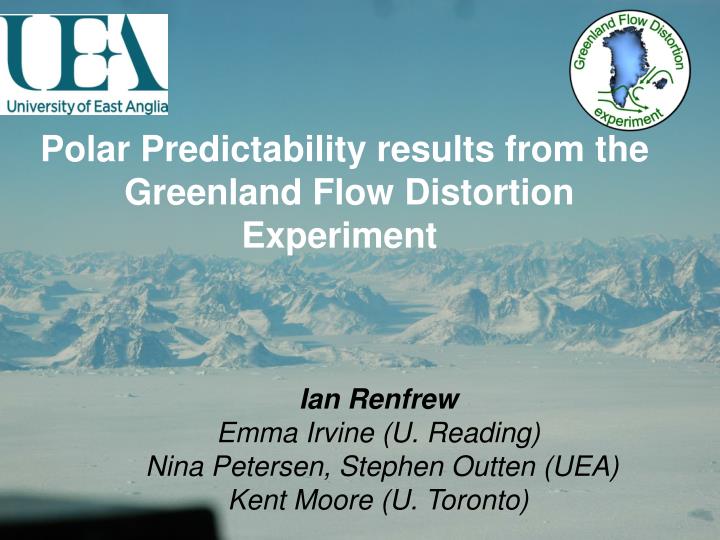
Polar Predictability results from the Greenland Flow Distortion Experiment . Ian Renfrew Emma Irvine (U. Reading) Nina Petersen, Stephen Outten (UEA) Kent Moore (U. Toronto). Outline. Motivation Short-range NWP improvements Case studies of tip jet & barrier winds

E N D
Polar Predictability results from the Greenland Flow Distortion Experiment Ian Renfrew Emma Irvine (U. Reading) Nina Petersen, Stephen Outten (UEA) Kent Moore (U. Toronto)
Outline Motivation Short-range NWP improvements Case studies of tip jet & barrier winds analyses validation Impact of Targeted Observations Conclusions
Motivation • Local weather systems • tip jets, barrier winds, lee cyclones, polar lows • Climate system • thermohaline circulation • Medium-range weather forecasting • targeted observations
QuikSCAT climatology Mean wind speed for DJF 1999-2004 Moore and Renfrew 2005, J. Climate
GFD: QuikSCAT climatology • (Westerly) Tip Jets Moore and Renfrew 2005, J. Climate
GFD: QuikSCAT climatology • Easterly Tip Jets Moore and Renfrew 2005, J. Climate
QuikSCAT climatology • Barrier winds Moore and Renfrew 2005, J. Climate
Field programme: 17 Feb – 12 March 2007 • Detachment: Keflavik, Iceland • 62 flight hours + 9 hours (EUFAR)
Results from case studies • Accurate NWP hindcast simulations required consideration of • Model setup, grid size, levels, etc • SST • Air-sea-ice interaction • PBL scheme • Examples: • Tip Jet (21 Feb 2007) • Barrier wind (1-6 March)
AVHRR Ch 1 14:35 UTC 21 February 2007
Easterly Tip Jet: 21 Feb • Met Office UM 6.1 • 12 km grid & 76 levels • Initialised from Met Office global analyses
Easterly Tip Jet: 21 Feb • Met Office UM 6.1 • 12 km grid & 76 levels • Initialised from Met Office global analyses • Configuration changes: • z0 over marginal ice zone changed 100mm → 0.5mm • z0 over sea ice changed 3mm → 0.5mm • OSTIA high resolution SST & sea-ice field See Outten et al. 2009,QJRMS Also Birch et al. 2009, J. Geophys. Res.
Easterly Tip Jet: 21 Feb Met Office UM 6.1 12 km grid & 76 levels Initialised from Met Office global analyses Configuration changes: z0 over marginal ice zone changed 100mm → 0.5mm z0 over sea ice changed 3mm → 0.5mm OSTIA high resolution SST & sea-ice field
Easterly Tip Jet: 21 Feb • Met Office UM 6.1 • 12 km grid & 76 levels • Initialised from Met Office global analyses • Configuration changes: • z0 over marginal ice zone changed 100mm → 0.5mm • z0 over sea ice changed 3mm → 0.5mm • OSTIA high resolution SST & sea-ice field • Reasonably accurate simulation: • 1-2 K and 2-3 m s-1 in ABL
Easterly Tip Jet: 21 Feb Met Office UM 6.1 12 km grid & 76 levels Initialised from Met Office global analyses Configuration changes: z0 over marginal ice zone changed 100mm → 0.5mm z0 over sea ice changed 3mm → 0.5mm OSTIA high resolution SST & sea-ice field Reasonably accurate simulation: 1-2 K and 2-3 m s-1 in ABL
Barrier Flows: 2 March 2007 DS North Cross-section DS South Cross-section
Barrier Flows: 2 March 2007 DS South Cross-section
Barrier Flows: Temperature inversions Sharp elevated temperature inversions not in analysis or forecasts Due to SBL over Greenland? Data assimilation will smooth out?
Barrier Flows: Summary • Synoptic situation controls wind speed maxima • Barrier effect doubles wind speed • UM simulations ok • Following sea-ice & SST changes • But fail to capture sharp temp. inversion See Petersen, Renfrew & Moore, 2009 QJRMS
Comparison of aircraft-based surface-layer observations over Denmark Strait and the Irminger Sea with meteorological analyses and QuikSCAT winds I. A. Renfrew, G. N. Petersen, D. A. J. Sproson, G. W. K. Moore, H. Adiwidjaja, S. Zhang, and R. North (2009, QJRMS)
Focus on ECMWF Analyses • Underestimates U10 at highest wind speeds.
ECMWF 1.125 deg has a T2m bias of -0.7 K • T511 has no bias.
Some ABL temperature discrepancies due to SST • At time 1 deg SST • Now OSTIA
Some ABL temperature discrepancies due to SST • At time 0.5 deg SST and sea ice fields • Now OSTIA
Surface turbulent fluxes are well-modelled, but scatter and biases result in relatively large rms errors.
ECMWF surface layer comparison • ECMWF model does not capture the highest wind speeds observed, despite an operational resolution of T799 and archived data at T511/N400 (∼40 km). • This suggests mesoscale atmospheric flow features are being ‘smoothed out’ in some way (see Chelton et al. 2006). • At T511/N400, the model produces good estimates for the surface-layer temperature and humidities, despite a large scatter in the SST. But at lower archived resolution (1.125 deg) a bias of −0.7 K in T2m is introduced. • The ECMWF surface turbulent fluxes correspond reasonably well with the observations
Targeted Observations in GFDex: • 4 flights • 7 -11 dropsondes per flight • Dropsondes sent to GTS and assimilated into operational 12Z forecasts
Targeted Observations in GFDex: • 4 flights • 7 -11 dropsondes per flight • Dropsondes sent to GTS and assimilated into operational 12Z forecasts • Analysing the results via hindcast experiments: • Met Office UM 6.1, 24km grid • 4D-VAR data assimilation scheme, 48km grid • North-Atlantic European domain • Control – routine obs. only • Targeted – routine obs. + targeted obs. (dropsondes) See Irvine et al. 2009, QJRMS – general results of all cases
Impact of dropsonde data on Greenland coast ORIGINAL DATASET (targeted sondes) MODIFIED DATASET (Replaced sondes on Greenland coast with sondes in Denmark Strait)
Forecast impact with modified dataset (no sondes on Greenland coast) dashed line = targeted sondes, solid line = all sondes dotted line = MODIFIED DATASET (no sondes near Greenland)
Why do the dropsondes on the Greenland coast degrade the forecast? Sonde data is spread along terrain-following model levels – up steep orography See Irvine et al (2010) MWR, in press Analysis increment in v resulting from assimilation of targeted sonde X = sonde location X 38
Conclusions • To simulate the high winds associated with polar mesoscale weather systems, a model resolution of order 10 km is necessary but is not sufficient; as appropriate ABL, surface layer and surface flux parameterizations are also crucial. • An accurate prescription of the SST & sea ice is essential. • In regions relatively close to the sea-ice edge, the current generation of NWP models still have problems in accurately simulating ABL temperature and humidity. • Global analyses products don’t appear able to capture highest wind speeds (e.g. U10 in ECMWF). • Targeted observations programme had modest impact on forecasts (5-10%); also highlighted problems with soundings near steep and high orography.
Case studies • Obs & dynamics of an easterly tip jet • Obs & modelling of a Greenland lee cyclone • Barrier flows & wakes around Greenland • Climatological studies • A climatology of westerly tip jets • Targeted Observations • Impact assessment in collaboration with Met Office • Air-sea interaction: • Turbulent flux observations • Comparison of obs & NWP models • High-resolution ocean simulations
Stochastic-dynamic example • Stochastic KE Backscatter scheme (Shutts 2005) • upscale influence of deep convection in mesoscale convective systems and the statistical uncertainty of orographic drag representations • Improves systematic error in the tropics & extratropics (Shutts, 2005, Berner et al. 2008). 400 127 km
Potential solution: Reject sonde data below 850hPa? Green line shows an increase in forecast improvement when dropsondes near Greenland have data below 850hPa rejected
Comparison of model data and sonde data near Greenland NW SE