Download

1 / 55
560 likes | 700 Views
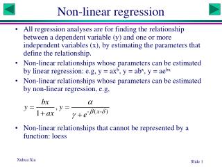
Non-Linear Models. Non-Linear Growth models. The Mechanistic Growth Model. many models cannot be transformed into a linear model. Equation :. or (ignoring e ) “rate of increase in Y” =. The Logistic Growth Model. Equation :. or (ignoring e ) “rate of increase in Y” =.

E N D
Non-Linear Growth models The Mechanistic Growth Model • many models cannot be transformed into a linear model Equation: or (ignoring e) “rate of increase in Y”=
The Logistic Growth Model Equation: or (ignoring e) “rate of increase in Y”=
The Gompertz Growth Model: Equation: or (ignoring e) “rate of increase in Y”=
Non-Linear Regression Introduction Previously we have fitted, by least squares, the General Linear model which were of the type: Y = b0 + b1X1 + b2 X2 + ... + bpXp + e
the above equation can represent a wide variety of relationships. • there are many situations in which a model of this form is not appropriate and too simple to represent the true relationship between the dependent (or response) variable Y and the independent (or predictor) variables X1 , X2 , ... and Xp. • When we are led to a model of nonlinear form, we would usually prefer to fit such a model whenever possible, rather than to fit an alternative, perhaps less realistic, linear model. • Any model which is not of the form given above will be called a nonlinear model.
This model will generally be of the form: Y = f(X1, X2, ..., Xp| q1, q2, ... , qq) + e * where the function (expression) f is known except for the q unknown parameters q1, q2, ... , qq.
Suppose that we have collected data on the Y, • (y1, y2, ...yn) • corresponding to n sets of values of the independent variables X1, X2, ... and Xp • (x11, x21, ..., xp1) , • (x12, x22, ..., xp2), • ... and • (x12, x22, ..., xp2).
For a set of possible values q1, q2, ... , qq of the parameters, a measure of how well these values fit the model described in equation * above is the residual sum of squares function • where • is the predicted value of the response variable yi from the values of the p independent variables x1i, x2i, ..., xpi using the model in equation * and the values of the parameters q1, q2, ... , qq.
The Least squares estimates of q1, q2, ... , qq, are values • which minimize S(q1, q2, ... , qq). • It can be shown that the error terms are independent normally distributed with mean 0 and common variance s2 than the least squares estimates are also the maximum likelihood estimate of q1, q2, ... , qq).
To find the least squares estimate we need to determine when all the derivatives S(q1, q2, ... , qq) with respect to each parameter q1, q2, ... and qq are equal to zero. • This quite often leads to a set of equations in q1, q2, ... and qq that are difficult to solve even with one parameter and a comparatively simple nonlinear model. • When more parameters are involved and the model is more complicated, the solution of the normal equations can be extremely difficult to obtain, and iterative methods must be employed.
To compound the difficulties it may happen that multiple solutions exist, corresponding to multiple stationary values of the function S(q1, q2, ... , qq). • When the model is linear, these equations form a set of linear equations in q1, q2, ... and qq which can be solved for the least squares estimates . • In addition the sum of squares function, S(q1, q2, ... , qq), is a quadratic function of the parameters and is constant on ellipsoidal surfaces centered at the least squares estimates .
Example We have collected data on two variables (Y, X) The model we will consider is Y = q1e-X +q2 + e The data: (x1 ,y1) (x2,y2) (x3,y3) , ... , (xn,yn)
The predicted value of yiusing the model is: The Residual Sum of Squares is: The least squares estimates of q1 and q2 satisfy
Techniques for Estimating the Parameters of a Nonlinear System • In some nonlinear problems it is convenient to determine equations (the Normal Equations) for the least squares estimates , • the values that minimize the sum of squares function, S(q1, q2, ... , qq). • These equations are nonlinear and it is usually necessary to develop an iterative technique for solving them.
In addition to this approach there are several currently employed methods available for obtaining the parameter estimates by a routine computer calculation. • We shall mention three of these: • 1) Steepest descent, • 2) Linearization, and • 3) Marquardt's procedure.
In each case a iterative procedure is used to find the least squares estimators . • That is an initial estimates, ,for these values are determined. • The procedure than finds successfully better estimates, that hopefully converge to the least squares estimates,
Steepest Descent • The steepest descent method focuses on determining the values of q1, q2, ... , qq that minimize the sum of squares function, S(q1, q2, ... , qq). • The basic idea is to determine from an initial point, and the tangent plane to S(q1, q2, ... , qq) at this point, the vector along which the function S(q1, q2, ... , qq) will be decreasing at the fastest rate. • The method of steepest descent than moves from this initial point along the direction of steepest descent until the value of S(q1, q2, ... , qq) stops decreasing.
It uses this point, as the next approximation to the value that minimizes S(q1, q2, ... , qq). • The procedure than continues until the successive approximation arrive at a point where the sum of squares function, S(q1, q2, ... , qq) is minimized. • At that point, the tangent plane to S(q1, q2, ... , qq) will be horizontal and there will be no direction of steepest descent.
It should be pointed out that the technique of steepest descent is a technique of great value in experimental work for finding stationary values of response surfaces. • While, theoretically, the steepest descent method will converge, it may do so in practice with agonizing slowness after some rapid initial progress.
Slow convergence is particularly likely when the S(q1, q2, ... , qq) contours are attenuated and banana-shaped (as they often are in practice), and it happens when the path of steepest descent zigzags slowly up a narrow ridge, each iteration bringing only a slight reduction in S(q1, q2, ... , qq).
A further disadvantage of the steepest descent method is that it is not scale invariant. • The indicated direction of movement changes if the scales of the variables are changed, unless all are changed by the same factor. • The steepest descent method is, on the whole, slightly less favored than the linearization method (described later) but will work satisfactorily for many nonlinear problems, especially if modifications are made to the basic technique.
Steepest Descent Steepest descent path Initial guess
Linearization • The linearization (or Taylor series) method uses the results of linear least squares in a succession of stages. • Suppose the postulated model is of the form: Y = f(X1, X2, ..., Xp| q1, q2, ... , qq) + e • Let be initial values for the parameters q1, q2, ... , qq. • These initial values may be intelligent guesses or preliminary estimates based on whatever information are available.
These initial values will, hopefully, be improved upon in the successive iterations to be described below. • The linearization method approximates f(X1, X2, ..., Xp| q1, q2, ... , qq) with a linear function of q1, q2, ... , qq using a Taylor series expansion of f(X1, X2, ..., Xp| q1, q2, ... , qq) about the point and curtailing the expansion at the first derivatives. • The method then uses the results of linear least squares to find values, that provide the least squares fit of of this linear function to the data .
The procedure is then repeated again until the successive approximations converge to hopefully at the least squares estimates:
Linearization Contours of RSS for linear approximatin 2nd guess Initial guess
3rd guess Contours of RSS for linear approximatin 2nd guess Initial guess
4th guess 3rd guess Contours of RSS for linear approximatin 2nd guess Initial guess
1. It may converge very slowly; that is, a very large number of iterations may be required before the solution stabilizes even though the sum of squares S(q1, q2 , …, qp) may decrease consistently as the number of iterations increase. This sort of behavior is not common but can occur. 2. It may oscillate widely, continually reversing direction, and often increasing, as well as decreasing the sum of squares. Nevertheless the solution may stabilize eventually. 3. It may not converge at all, and even diverge, so that the sum of squares increases iteration after iteration without bound. The linearization procedure has the following possible drawbacks:
The linearization method is, in general, a useful one and will successfully solve many nonlinear problems. • Where it does not, consideration should be given to reparameterization of the model or to the use of Marquardt's procedure.
Example Non-Linear Regression
7 days after application • 14 days after application • 21 days after application • 28 days after application • 42 days after application • 56 days after application • 70 days after application • 84 days after application In this example we are measuring the amount of a compound in the soil:
Craik • Tilson This is carried out at two test plot locations 6 measurements per location are made each time
Some starting values of the parameters found by trial and error by Excel
ANOVA Table (Craik) Parameter Estimates (Craik)
Testing Hypothesis: similar to linear regression Caution: This statistic has only an approximate F – distribution when the sample size is large
Example: Suppose we want to test H0: c = 0 against HA: c ≠ 0 Complete model Reduced model
ANOVA Table (Complete model) ANOVA Table (Reduced model)
Use of Dummy Variables Non Linear Regression
The Model: or where