Download
1 / 24
240 likes | 349 Views
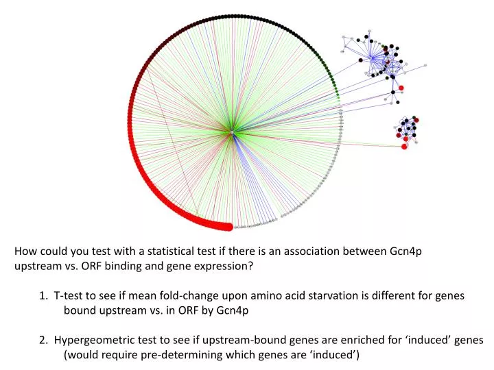
How could you test with a statistical test if there is an association between Gcn4p upstream vs. ORF binding and gene expression? 1. T-test to see if mean fold-change upon amino acid starvation is different for genes bound upstream vs. in ORF by Gcn4p

E N D
How could you test with a statistical test if there is an association between Gcn4p upstream vs. ORF binding and gene expression? 1. T-test to see if mean fold-change upon amino acid starvation is different for genes bound upstream vs. in ORF by Gcn4p 2. Hypergeometric test to see if upstream-bound genes are enriched for ‘induced’ genes (would require pre-determining which genes are ‘induced’)
Genetic mapping: linking phenotype to genotype Lab studies of gene knockouts, RNAi, and mutagenesis screens can reveal phenotypes A major goal is to do the reverse: use natural phenotypic variation to identify causal variants reveals phenotypic and genetic variation relevant in ‘the wild’ Goal: Identify QTL(Quantitative Trait Locus) or QTN (Quantitative Trait Nucleotide) that significantly correlate with (and there likely explain) the phenotype
Two strategies for genetic mapping Linkage Mapping Association Mapping (GWAS) Mate two parents with opposite phenotypes and score progeny Score many individuals from natural (randomly mating) populations Ability to identify QTL/QTLs requires recombination to mix and match the genomes. Linkage mapping: generate recombination through crosses. Generally need many individuals (or many generations: increased recombination frequency = smaller regions) Association mapping: uses historical recombination events between individuals. Generally requires fewer individuals for the same statistical power.
Goals of QTL linkage mapping • To identify the loci that contribute to phenotypic variation • Cross two parents with extreme phenotypes • Phenotype all the progeny • Genotype the progeny at markers across the genome • Associate the observed phenotypic variation with the underlying genetic variation • Ultimate goal: identify causal polymorphisms that explain the phenotypic variation Ades 2008, NHGRI
Backcross Phenotype: Drug tolerance 80% 20% viability Usually have at least 100 individuals Broman and Sen 2009
Intercross Phenotype: Drug tolerance 80% 20% viability Can reveal AA, BB, and AB genotypes. Takes more individuals to map, due to more intricate genotypes generated Broman and Sen 2009
Genetic map: specific markersspaced across the genome • Markers can be: • SNPs at particular loci • Variable-length repeats • e.g. ALU repeats • ALL polymorphisms • (if have whole genomes) Ideally, markers should be spaced every 10-20 cM and span the whole genome
Genotype data: Determine allele at all markers in each F2 Phenotype: e.g. drug tolerance score
Statistical framework • Missing Data Problem • Use marker data to infer intervening genotypes • 2. Model Selection Problem • How do the QTL across the genome combine with the covariates to generate the phenotype? Broman and Sen 2009
Marker regression: simple T-test (or ANOVA) at each marker Marker 1: no QTL Marker 2: significant QTL (population means are different)
Marker regression Advantages: • Simple test – standard T-test/ANOVA • Covariates (e.g. Gender, Environment) are to incorporate • No genetic map necessary, since test is done separately on each marker Disadvantages: • Any individuals with missing marker data must be omitted from analysis • Does not effectively consider positions between markers • Does not test for genetic interactions (e.g. epistasis) • The effect size of the QTL (i.e. power to detect QTL) is reduced by incomplete • linkage to the marker • Difficult to pinpoint QTL position, since only the marker positions are considered
Interval mapping • Lander and Botstein 1989 • In addition to examining phenotype-genotype associations at markers, look for associations between makers by inferring the genotype A A A A Q • The methods for calculating genotype probabilities between markers typically use hidden Markov models to account for additional factors, such as genotyping errors
Interval mapping Advantages: • Takes account of missing genotype information – all individuals are included • Can scan for QTL at locations in between markers • QTL effects are better estimated Disadvantages: • More computation time required • Still only a single-QTL model – cannot separate linked QTL or examine for interactions among QTL
LOD scores • Measure of the strength of evidence for the presence of a QTL • at each marker location LOD(λ) = log10 likelihood ratio comparing the hypothesis of a QTL at position λ versus that of no QTL } { Pr(y|QTL at λ, µAAλ,µABλ,σλ) log10 Pr(y|no QTL, µ,σ) LOD 3 means that the TOP modelis 103 times more likely than the BOTTOM model Phenotype
LOD curves Chromosome How do you know which peaks are really significant?
LOD threshold • Consider the null hypothesis that there are no QTLs genome-wide one location genome-wide Randomize the phenotype labels on the relative to the genotypes Conduct interval mapping and determine what the maximum LOD score is genome-wide Repeat a large number of times (1000-10,000) to generate a null distribution of maximum LOD scores Broman and Sen 2009
LOD threshold • 1000 permutations • 10% False Discovery Rate = LOD 3.19 • (means that at this LOD cutoff 10% of peaks could be random chance) • 5% FDR = LOD 3.52 • Boundary of the peak is often taken as points that cross (Max LOD – 1.5) (or - 1.8 for an intercross)
Association Mapping Haplotype blocks: linked alleles segregating together means that only subsets of SNPs need to be genotyped. Relies on historic matings in “randomly mating” populations. Most populations are not randomly mating – therefore need to consider population structure.
TASSEL: Trait Analysis by aSSociation, Evolution and Linkage Bradbury et al. (Buckler Lab) Genotypes for 65 strains Phenotypes for 65 strains Phylogenetic Relatedness Population Structure Random Error Random Error Strains Dana Wohlbach
Association Mapping FDR threshold set by permutation analysis or q value correction -log p-value
Meta-analysis of 15 GWAS studies of IBD = 75,000 people. - Imputation-based GWAS: imputed SNPs where there was missing data (using known haplotypes and human HapMap3 reference data) - Identified 25,075 SNPs that were significantly associated with IBD (p < 0.01) … collapsed these into 163 IBD-associated loci * 71 of these are new, due to increased statistical power * 163 loci is “far more” than associated with any other complex disease * More SNPs are linked to non-coding/regulatory variation than missense - Significant overlap with SNPs linked to immunodeficiences & bacterial infection - 13.6% of the phenotypic variance is explained by all these loci together
The challenge with human GWAS: missing heritability >1200 variants associated with ~165 complex human diseases. In most cases, known loci account for only 20-30% of the heritable phenotypic variance. PNAS 2011 They argue much of the “missing” heritability is not really missing: additive interactions (without considering epistasis) can only account for so much …
Investigating Epistasis: Genetic Interactions? Significant SNP (FDR 1%) Insignificant SNP How much of ‘missing’ heritability is explained by epistasis? Linear model for each pair of significant SNPs Dana Wohlbach
Many significant interactions between SNPs Significant SNP (FDR 1%) Insignificant SNP Significant interaction at: • 0.1% FDR (82 pairs) • 1.0% FDR (413 pairs) • Genetic or Physical (SGD) Dana Wohlbach