Download
1 / 58
580 likes | 733 Views
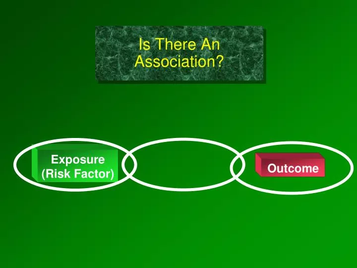
Is There An Association?. Exposure (Risk Factor). Outcome. Testing Whether a Factor Is Associated With Disease. Target Population. Inference. Sample. Are the results valid? Chance Bias Confounding. Study population. Collect data Make comparisons. Is there an association?.

E N D
Is There An Association? Exposure (Risk Factor) Outcome
Testing Whether a Factor Is Associated With Disease Target Population Inference Sample • Are the results valid? • Chance • Bias • Confounding Study population • Collect data • Make comparisons Is there an association?
Diseased & Exposed Diseased & non-exposed Non-diseased & exposed Non-diseased & non-exposed
Yes No Yes No • Cohort • Clinical Trial • Case-Control All Three Of These Can Be Summarized by a 2x2 Table Outcome Exposed? All three analytical studies rely on a comparison of groups to determine whether there is an association.
Yes No 7 124 131 Yes 1 78 79 No Wound Infection Incidental Appendectomy How many ways can we compare the groups? How would you interpret the comparisons?
For Cohort Type Studies Options For Comparing Incidence Ie I0 • Calculate the ratio of the incidences for the two groups. (Divide incidence in exposed group by the incidence in the control group). Or 2) Calculate the difference in incidence between the two groups. (Subtract incidence in control group from the incidence in the exposed group). Ie- I0
Risk Ratio Wound Infection Cumulative Incidence Yes No 5.3% Yes 7 124 131 (7/131) Had Incidental Appendectomy 1.3% No 1 78 79 (1/79) 8 202 210 Subjects “Risk Ratio” or “Relative Risk” RR = 7/131 = 5.3 = 4.2 1/79 1.3
5.3% Also had appendectomy 5.3% 1.3% RR = = = 4.2 1.3% No appendectomy Risk Ratio in Appendectomy Study A ratio; no dimensions. Interpretation: “In this study those who had an incidental appendectomy had 4.2 times the risk compared to those who did not have appendectomy.”
5.3% Exposed group 5.3% Unexposed group What If Risk Ratio = 1.0 ? 5.3% RR = = = 1.0 5.3%
139 10,898 11,037 exposed 239 10,795 11,034 not exposed What If Relative Risk < 1.0 ? Myocardial Infarction Yes No Yes Aspirin Use No 378 21,693 22,071 subjects Iexposed = 139/11,037 = .0126 Iunexposed = 239/11034 = .0221 RR = .0126 = 0.55 .0221
139 10,898 11,037 239 10,795 11,034 Interpretation of Relative Risk < 1.0 Myocardial Infarction Yes No Yes Aspirin Use No 378 21,693 22,071 “Subjects who used aspirin had 0.55 times the risk of myocardial infarction compared to those who did not use aspirin.” RR = .0126 = 0.55 .0221
Data Summary for Incidence Rate Disease Total Disease-free Obs. Time Yes No IR a/PY1 Yes a - PY1 Exposure c/PY0 No c - PY0 Relative risk = a/PY1 c/PY0 “Rate Ratio” or “Relative Risk”
Coronary Artery Disease Yes No Person-Years of Follow Up 30 - 54,308.7 Yes Postmenopausal Hormones 60 - 51,477.5 No 90 105,786.2 Incidence In treated group = 30 / 54,308.7 = 55.2 / 100,000 P-Yrs In untreated group = 60 / 51,477.5 = 116.6 / 100,000 P-Yrs Rate Ratio = 55.2 /100,000 P-Yr.= 55.2 = 0.47 116.6 /100,000 P-Yr. 116.6
It is more precise to say that postmenopausal women on HRT had 0.47 times the rate of coronary disease, compared to women not taking HRT. In practice, however, many people interpret it just like a risk ratio.
Multiple Exposure Categories Magnetic Field Exposure Cumulative Incidence 2,264/67,424=.0336 61/1,469 =.0415 30/674 =.0445 Low Medium High Risk Ratios .0336/.0336=1.00 .0415/.0336=1.23 .0445/.0336=1.33
? Non-fatal Myocardial Infarction Obesity Rate of MI per 100,000 P-Yrs (incidence) wgt kg hgt m2 # MIs (non-fatal) Person-years of observation Rate Ratio BMI: 41 177,356 23.1 1.0 <21 57 194,243 29.3 1.3 21-23 56 155,717 36.0 1.6 23-25 67 148,541 45.1 2.0 25-29 85 99,573 85.4 3.7 >29 The Nurse’s Health Study Multiple Exposure Categories - An “r x c” (row/column) Table ?
The Risk Difference (Attributable Risk) RD = Incidence in exposed - Incidence in unexposed Risk Difference = Ie - I0
Risk Difference in Appendectomy Study Wound Infection Cumulative Incidence Yes No 5.3% Yes 7 124 131 Had Incidental Appendectomy 1.3% No 1 78 79 8 202 210 subjects RD = 0.053 – 0.013 = 0.04 = 4 per 100
1.3/100 Risk Difference Gives a Different Perspective on the Same Information 5.3/100 Excess risk is 4 per 100 Adding an appendectomy appears to increase the risk by (4 per 100 appendectomies), so ... Even if appendectomy is not done, there is a risk of wound infection (1.3 per 100). Exposed Not Exposed … the RD is theexcess riskin those who have the factor, i.e., the risk of wound infection that can beattributedto having an appendectomy, assuming there is a cause-effect relationship.
Tip #1 for Interpretation of Risk Difference Convert % to convenient fractions to interpret for a group of people. Example: Incidence with appendectomy = 5.3% = 0.053 Incidence without appendectomy = 1.3% = 0.013 Risk Difference= 0.040 = 40/1000 i.e., 4 per 100 incidental appendectomies or 40 per 1,000 incidental appendectomies Interpretation: In the group that underwent incidental appendectomy there were 40 excess wound infection per 1000 subjects (or 4 per 100).
Tip #2 for Interpretation of Risk Difference The focus is on the excess disease in the exposed group. Interpretation: In the group with incidental appendectomy there were 4 excess wound infections per 100 subjects. This implies that if incidental appendectomy were performed on another 1,000 subjects having staging surgery, we would expect 40 excess wound infections attributable to the incidental appendectomy.
Tip #3 for Interpretation of Risk Difference Don’t forget to specify the time period when you are describing RD for cumulative incidence. Interpretation: In the group that failed to adhere closely to the Mediterranean diet there were 120 excess deaths per 1,000 men during a two year period of observation. In the appendectomy study the time period was very brief and was implicit (“postoperatively”) it wasn’t necessary to specify the time frame. However, for most cohort studies it is important. Remember that with cumulative incidence, the time interval is described in words.
wgt kg hgt m2 # MIs (non-fatal) Person-years of observation Relative Risk BMI: 41 177,356 1.0 <21 57 194,243 1.3 21-23 56 155,717 1.6 23-25 67 148,541 2.0 25-29 85 99,573 3.7 >29 Rate Differences Rate of MI per 100,000 P-Yrs (incidence) 23.1 29.3 36.0 45.1 85.4 Risk Difference= 85.4/100,000 - 23.1/100,000 = 62.3 excess cases / 100,000 P-Y in the heaviest group
Rate Difference Interpretation Among the heaviest women there were 62 excess cases of heart disease per 100,000 person-years of follow up that could be attributed to their excess weight. This suggests that if we followed 50,000 women with BMI > 29 for 2 years we might expect 62 excess myocardial infarctions due to their weight. (Or one could prevent 62 deaths by getting them to reduce their weight.) or If 100,000 obese women had remained lean, it would prevent 62 myocardial infarctions per year.
Influenza Vaccination and Reduction in Hospitalizations for Cardiac Disease and Stroke among the Elderly. Kristin Nichol et al.: NEJM 2003;348:1322-32. These investigators used the administrative data bases of three large managed care organizations to study the impact of vaccination in the elderly on hospitalization and death. Administrative records were used to whether subjects had received influenza vaccine and whether they were hospitalized or died during the year of study. The table below summarizes findings during the 1998-1999 flu season.
If the exposure is vaccination & outcome of interest is death, what is the risk difference? 77,738 62,217 RD = CIe – CIu = (943 / 77,738) - (1,361 / 62,317) = -0.0097 = - 97/10,000 over a year
Can a risk difference be a negative number? -97/10,000 over a year Instead of calling it ‘excess risk’, just refer to it as a ‘risk reduction.’
RR & RD Provide Different Perspectives • Risk Difference:a better measure ofpublic health impact. • How much impact would prevention have? • How many people would benefit? Relative Risk:shows thestrengthof the association. • RR = 1.0 suggests no association • RR close to 1.0 suggests weak association • RR >> 1.0 or RR << 1.0 suggests a strong association
A large study looked at whether fecal occult blood testing (FOBT) could decrease mortality from colorectal cancer (CRC). FOBT Relative Risk Perspective: FOBT decreased mortality from CRC by 33% ! (RR = .67 for FOBT compared to no screening) Risk Difference Perspective: FOBT decreased mortality from 9 per 1,000 people to 6 per 1,000. So, RR= 0.67 (i.e., 0.006/0.009 BUT The risk difference was only 3 per 1,000 people screened. The ratio of these two numbers is more impressive than the actual difference.
Calculate RR & RD for Two Diseases Annual Mortality per 100,000 (CI) Lung Cancer Cigarette smokers140 Non-smokers 10 RR= 14 RD= 130 per 100,000 Annual Mortality per 100,000 (CI) Coronary Heart Disease Cigarette smokers669 Non-smokers 413 RR= 1.6 RD= 256 per 100,000 Smoking is a stronger risk factor for …. ? Smoking is a bigger public health problem for …. ?
Smokers Non-smokers Smokers Non-smokers
Aspirin & MI Aspirin Placebo RR (/10,000) (/10,000) 0.59 What should we conclude? What should we recommend?
Benefits & Risks Aspirin Placebo RR (/10,000) (/10,000) 0.59 What should we conclude? What should we recommend?
Benefits & Risks Aspirin Placebo RR RD (/10,000) (/10,000) (/10,000)
If we are going to discuss rare, but serious possible complications of influenza vaccine, would it be better to look at the Risk Ratio or the Risk Difference? Observed frequency in: Exposed people: 2 / 100,000 Unexposed people: 1 / 100,000 Risk Ratio = 2; those exposed had two times the risk! (OMG!) Risk Difference = 1 per 100,000; assuming that the exposure is a cause of the outcome, the exposed group had an excess risk of 1 case per 100,000 subjects.
Attributable Risk % - The Attributable Proportion The proportion (%) of disease in the exposed group that can be attributed to the exposure, i.e., the proportion of disease in the exposed group that could be prevented by eliminating the risk factor. AR% = RD x 100 Ie .04 .053 .013 .04 x 100 = 75% .053 What % of infections in the exposed group can be attributed to having the exposure? Not Exposed Exposed Interpretation: 75% of infections in the exposed group could be attributed to doing an incidental appendectomy.
Consider this cohort study conducted over 1 year: Total risk in exposed group? 0.050 = 50/1,000 Excess risk in exposed group? 0.050 – 0.10 = 40/1,000 over 1 yr. Attributable proportion in exposed group? 40/1,000 = 80% 50/1,000
The Population Attributable Proportion Of the 1,400 diseased people, only 500 were exposed (35.7%). Of these only 80% can be attributed to the exposure. So, in the total population the fraction of cases that can be attributed to the exposure is 0.357 x 0.80 = 0.286, or 28.6%.
cases (Already have disease) Odds of having the risk factor prior to disease? controls (No disease) But in a case-control study we find diseased and non-diseased people and we measure and compare the prevalence of prior exposures. To calculate incidence, you need to take a group of disease-free people and measure the occurrence of disease over time.
How many exposed people did it take to generate the 7 cases in the 1st cell? Cohort Study Wound Infection Cumulative Incidence Yes No 5.3% Yes 7 124 131 Had Incidental Appendectomy 1.3% No 1 78 79 Probability that an exposed person had disease? Odds that an exposed person had disease?
Control Case Hepatitis Case-Control Study Yes No ? 18 7 Yes In a true case-control study, you do not know the denominators for exposure groups! Ate at Deli ? 1 29 No 19 36 How many people had to eat at the Deli in order to generate the 18 cases in the 1st cell?
If the outcome is uncommon, the odds of exposure among non-disease subjects will be similar to the odds of exposure among the total population… So the odds ratio will be a good estimate of the risk ratio. (7/1,000) = Odds Ratio (7/1,007) = Risk Ratio (6/5,634) (6/5,640)
(7/1,000) = Odds Ratio (7/1,007) = Risk Ratio (6/5,634) (6/5,640) But this rearranges algebraically: 7 5,634 (7 / 1,000) 7 5,634 (7 / 6) x = = = x 6 1,000 (6 / 5,634) 1,000 6 (1,000 / 5,634) Odds of exposure in Disease Odds of exposure in Non-Disease Odds of disease in Exposed Odds of disease in Unexposed
Hepatitis Yes No 18 7 Yes Control Case Ate at Deli 1 29 No Odds of Disease Odds of Exposure Deli =18/7 No Deli =1/29 In cases =18/1 In controls =7/29 = 75 = 75
An Odds Ratio Is Interpreted Like Relative Risk An odds ratio is a good estimate of relative risk when the outcome is relatively uncommon. The odds ratio exaggerates relative risk when the outcome is more common. “Individuals who ate at the Deli had 75 times the risk of hepatitis A compared to those who did not eat at the Deli.”
You can always calculate an odds ratio, but… In cohort studies and clinical trials you can calculate incidence, so you can calculate either a relative risk or an odds ratio. In a case-control study, you can onlycalculate an odds ratio.
Yes No Not Cohort Design: Calculate RR or OR Kid pool Compare frequency of Giardia Got Giardiasis Yes No 16 108 124 Exposed to Kiddy Pool 14 341 355 I can compute either RR or OR here. Why?
Giardia Cumulative Incidence Yes No 16 / (16+108) = 12.9% 14 / (14+341) = 3.9% Not 16 108 Kid pool vs. 14 341 Risk Ratio = 3.3 Odds = 16/14 Ratio 108/341 = 3.6
Calculation of the Odds Ratio Ratio of Odds of Disease Ratio of Odds of Exposure Cross Product Odds = 16/108 Ratio 14/341 = 3.6 Odds = 16/14 Ratio 108/341 = 3.6 Odds = 16x341 Ratio 108x14 = 3.6 16 108 Kid pool b a vs. 14 341 Not d c a/b c/d a/c b/d a x d b x c = =