Download
1 / 70
700 likes | 882 Views
Climate Change Observed and Projected. Jim Zandlo State Climatology Office - DNR – EcoWaters MN Forest Resources Council Meeting March 23, 2011. Observable Climate Changes. Rates of changes in time have generally intensified since about 1980. Temperatures warming Precipitation increasing

E N D
Climate ChangeObserved and Projected Jim Zandlo State Climatology Office - DNR – EcoWaters MN Forest Resources Council Meeting March 23, 2011
Observable Climate Changes Rates of changes in time have generally intensified since about 1980. • Temperatures warming • Precipitation increasing • Some precipitation conditions returning to conditions of about 100 years ago. • Other conditions affected by changing climate • Lake ice dates and water temperature • Streamflow? • Other ‘natural resources’? Caveats • Over longer time periods not as ‘one-sided’. • Non-climatic influences in the data
Temperature • Increasing everywhere • more in north (top 1/3 of Minnesota) • more rapidly recently (since 1980) • more at night (Tminimum) • more in winter (Dec-Feb) • Maps of observed warming of the last decade show warming everywhere. Some hint of extra warming around urbanizing locations. • Water temperature of Lake Superior warming as well.
‘Non-climatic’ influences • Local climate change • Equipment bias • Site bias • Measurement contamination • Observational errors • Transcription error (data entry) • Time-of-observation bias • Global climate change
‘Non-climatic’ influences • Local climate change • Land-use • Urbanization • Forest regrowth, conversion • Agricultural practice • No-till • Irrigation or not http://duckwater.bu.edu/urban/sprawl.jpg
‘Non-climatic’ influences • Site bias change • ‘minor’ station moves • 100 feet elevation, 5 miles allowed • ‘minor’ equipment moves ‘on-site’ • Site exposure • Tree growth • Buildings, roads, other infrastructure added
‘Non-climatic’ influences • Site bias change • ‘minor’ station moves [H1,SL] • 100 feet elevation, 5 miles allowed • ‘minor’ equipment moves ‘on-site’ • Site exposure • Tree growth • Buildings, roads, other infrastructure added
‘Non-climatic’ influences • Time-of-observation bias
Atmospheric Humidity • Average dewpoint temperature is up slightly in summer, in winter dropping until about 1980 then recent rapid rise. • Rising temperatures impacts may be amplified by rising air heat content due to humidity. • Number of very humid days (Tdew>70) rising rapidily in last few decades but was as high in the 1940s. • Summer dewpoints dropping off less at night.
Precipitation, Snow, Snow Depth • Increasing since 1930s ‘dust bowl’ years. • ‘below normal’ year unusual since 1990. • Number of heavy rain events increasing for decades but was as high a century ago. • Snow fall generally increasing but recently decreasing in south.
Lake Ice Out Dates • Trend toward earlier dates has been increasing • Pattern of ice out dates across the state is 3-4 days earlier now than it was about 35 years ago.
Some existing ‘future climate’ tools
Adopted from: http://en.wikipedia.org/wiki/Special_Report_on_Emissions_Scenarios
The Modeled Futuresome examples of tools and ‘data’ • IPCC reports http://www.ipcc.ch/ • Statistically downscaled monthly GCM * • The data http://gdo-dcp.ucllnl.org/ • Summary maps; Climate Wizard http://www.climatewizard.org/ • Dynamically downscaled GCM * • NARCCAPhttp://www.narccap.ucar.edu/ • All the GCM output * • PCMDI (info) http://www-pcmdi.llnl.gov/ipcc/about_ipcc.php • ESG (downloads) https://esg.llnl.gov:8443/index.jsp • Model host specific websites • SDSM Statistical DownScalingModel https://co-public.lboro.ac.uk/cocwd/SDSM/ • Panoply netCDF viewer * http://www.giss.nasa.gov/tools/panoply/ • ‘Climate Scenario at a Place’ [in Minnesota] http://climate.umn.edu/mapClim2007/tsSc.asp * All GCM, including downscaled, model time series data is distributed in netCDF format. Windows programs, s.a. Excel, don’t ‘know it’. A viewer or ability to write computer code is required for use. Some ESRI products may have ability to use netCDF. A single netCDF file is typically hundreds of Mb, commonly a Gb or more. There are hundreds of netCDF files available.
Pretty big picture projections … Average of 19 climate models. www.ldeo.columbia.edu/res/div/ocp/drought/science.shtml Global Climate Change Impacts in the United States. www.globalchange.gov/usimpacts
IPCC AR4 A1B projections from 21 models 2080 to 2099 1980 to 1999 • ‘Projections’ of past conditions • missed temperature by -4.1 to 3.5 • missed precipitation by -37% to +84%
‘Downscale’ for local detail … Regional climate change adaptation strategies for biodiversity conservation in a midcontinental region of North America 2009 Susan Galatowitsch, Lee Frelich, Laura Phillips-Mao
2009 Susan Galatowitsch, Lee Frelich, Laura Phillips-Mao Geographic Analogies: Places where the current climate resembles the climate projected for the future.
Climate Data for Climate Change Adaptation Analyses Jim Zandlo State Climatology Office – DNR Waters DNR climate Change Adaptation Scoping Discussion November 24, 2009
The Modeled Future • What’s needed for addressing adaptation issues? • summary of changes for some specific date or the trend over time relative to a base period. • time series used to emulate what’s affected • General Circulation Models (GCMs) • used for globalclimatemodeling • complicated • time series of future climatic conditions
The Modeled Future • General Circulation Models (GCMs) • Time series use • ‘raw’ • Downscaled • Statistical • Dynamic (regional climate models) • Statistics use • Trends and differences • derived time series • Analogy (past observations that look like modeled future) • Stochastic (weather generator)
What is needed from the ‘data’ for adaptation studies? • Summary of changes for some specific date or the trend over time relative to a base period. • e.g. 5°F warmer in 2050 than 1970-2000 • e.g. a graph (time series) of relative changes. • Time series used to emulate what’s affected • annual, monthly, daily, even sub-daily available • GCM model ‘data’ generally has biases • Use in ‘applied’ model; e.g. fish survival
The Modeled Future • Many General Circulation Models (GCMs) which are used for globalclimatemodeling. • Many institutions have their own models • Many scenarios of the future conditions that we ‘control’ • Many starting points (‘initial conditions’) for calculations
Adopted from: http://en.wikipedia.org/wiki/Special_Report_on_Emissions_Scenarios
Data Availability WCRP CMIP3 - http://www-pcmdi.llnl.gov/ipcc/about_ipcc.php ‘World Climate Research Programme – Coupled Model Intercomparison Project’
http://www.fs.fed.us/rmrs/docs/climate-change/western-watersheds-workshop/climate-models-scenarios.pdfhttp://www.fs.fed.us/rmrs/docs/climate-change/western-watersheds-workshop/climate-models-scenarios.pdf
The Modeled Future:Uncertainty • ‘Que sera, sera’ – things will change, we’re just not sure how • Model differences: unresolved science • Intrinsic (initial conditions) Presented by Ben Santer, Portland 2009
Example of initial condition uncertainty Simulated and observed regional sea-surface temperatures courtesy Ben Santer 1900 1920 1940 1960 1980 2000 40
Computer models can perform the “control experiment” that we can’t do in the real world < notice ‘anomoly’ scale (around zero) Average surface temperature change (°C) Meehlet al., Journal of Climate (2004) as presented by Ben Santer, Portland 2009
The Modeled Future (past) • GCMs are judged by how well their calculations of the climate of some recent period (e.g. 1970-2000) compare to what was measured. • Trends: match well • Absolute values and (?) statistical distribution: ‘not so much’
PowerPointPDF - A method of correction of regional climate model data for hydrological modelling, Juris Sennikovs, Uldis Bethers
What is Downscaling? Something you do to a 20th-Century climate model simulation to reproduce the observed climate. Will also give the projected regional climate change when applied to a future climate model simulation. From Salathe, Portland 2009
An Example: hydrology models Need runoff (RO) • Daily or even sub-daily required • Highly non-linear response • RO zero or very small unless a precip threshold is reached • Heavy RO only occurs for largest precip events • GCM models • Precip is average over a large area. But, averages over large areas, of course, are always no bigger and generally much smaller than amounts that fell at any given point within the area. • Readily available ‘downscaled’ GCM data currently only on a monthly time scale (same sort of problem as with areal averages; i.e. what happened over a smaller slice of time such as a day?). That is, the GCM estimates of future conditions cannot be used ‘as is’ by someone using long-standing existing hydrologic modeling techniques.
In a 1°x2° GCM grid cell (thousands of square miles) a single value for precipitation is calculated.
In a 1°x2° GCM grid cell (thousands of square miles) a single value for precipitation is calculated. An intense storm can have precipitation changes of as much as one inch per mile.
In a 1°x2° GCM grid cell (thousands of square miles) a single value for precipitation is calculated. An intense storm can have precipitation changes of as much as one inch per mile. 6 inches of rain is readily handled by a ‘100 year design’ culvert but 16 inches will wash it away.
Hokah ann max daily PRCP vs. RP precipitation, inches return period (years)