Algorithm for LAT On-board / On-ground GRB Trigger and Localization Jay Norris

1. Algorithm for LAT On-board / On-ground GRB Trigger and Localization Jay Norris

2. The Detection Problems - 1 On-ground Detection: • Near threshold: GRB signal (5-10 ’s, 40 s, > 50 MeV), with 2 Hz bckgnd rate  1/300 count -1 (  = sq. deg.), or 2 counts in 15° radius. • For extended emission (~ 103 s) in a bright burst, the corresponding bckgnd total is ~ 50 counts, perhaps comparable to the signal. Recourse: more severe cuts, probably removing more low-energy signal. Use Likelihood. • Notes: • “2 Hz bckgnd” means total sky rate: sources + extragalactic & galactic diffuse + residual particle bckgnd. (Possibly higher with looser cuts for maximum GRB signal.)

3. On-board Triggering: • At threshold, GRB signal ~ 5-10 ’s in 20-40 s (>50 MeV) • Bckgnd rate ~ 600 Hz  40 s / 41,253  ~ 0.6 count -1 • Suppose GBM 2 radius ~ 10°  190 bckgnd count -1 total in 40 s. Knowing GBM position facilitates on-board ID’ing of LAT GRB photons, but clearly … • A localization will require additional cleverly divined filters applied to a GRB event buffer, to reduce the rate to ~ 60 Hz  20 bckgnd counts (further reducible on-board). • This is a “worthy goal” for the on-board GRB filter chore. The Detection Problems - 2

4. Straightforward LAT GRB Detection & Localization Algorithm Philosophy (On-ground analysis): • Usually, negligible bckgnd and only one source (the GRB) • High-energy ’s provide accuracy, but are less numerous. • More low-energy ’s, and they are “bunched in time.” •  Optimal algorithm should be unbinned in time (thereby exploit bunching) and in space (exploit high-energy ’s).* • Starting from all-sky sample, algorithm should be able to bootstrap GRB position with very few false positives. • *This same conclusion applies for on-board trigger/localization, but it is constraint of GBM position (rather than ground filters) that lowers the bckgnd rate sufficiently, AND pinpoints GRB onset (thereby greatly reducing Ntrials).

5. Event with smallest s {s} : distances {t} : intervals Swift/BAT z = 0.547

6. Algorithm • An N-event sliding window is used as the bootstrap step in searching for significant temporal-spatial clustering. Compute the Log {Joint (spatial*temporal) likelihood} for the tightest spatial cluster of events in the temporal sliding window: Log(P) =  Log{ [1 – cos(di)] / [1 – cos(max)] } +  Log{ 1 – exp(-Rti) } • Log(P) is measured against the near real-time bckgnd rate (R). Trigger threshold is also set as a function of the bckgnd, such that high GRB trigger efficiency is realized (events w/ 5-10 ’s detected), and formal expectation for false positive < 10-6/day. • Localization algorithm collects all events between 1st and last windows which trigger within a time limit, ~ 150 s; computes an energy-weighted centroid. Probable particle events are ID’ed—by virtue of difference between actual and predicted distances from centroid—and then deweighted. Convergence: one iteration.

7. Implementation On-board Trigger and Localization Sequence: • Send LAT telemetry event stream to GRB processor. • Apply additional filters, reduce background rate to ~ 60 Hz. • Run spatial/temporal sliding-window trigger/localization algorithm. • Option to utilize GBM trigger time and position to reduce windows. • Telemeter localization and other GRB information to ground. • Option to send alert message with ~ 10 highest energy GRB events to ground for rapid localization analysis. Some Adjustable/Variable Parameters: • On-board / On-ground filters • Nevents in sliding window(s); Nmove events per trial • GBM positional uncertainty • Inclusion radius ( threshold energy) for GRB ’s • “This” trigger-active search interval • Trigger threshold(s) • Nsigma distance threshold for deweighting putative particle events

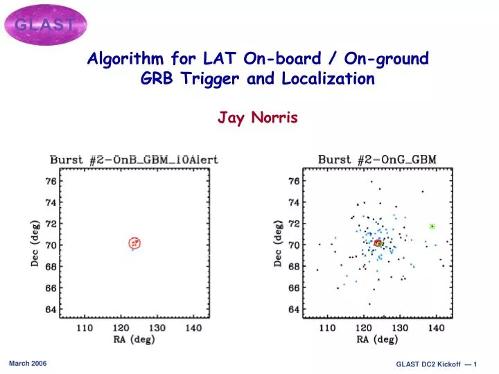
8. Red Circle: 10  est Bckgnd rate = 32 Hz, 60-event sliding window Burst 2 Localization from 10 events telemetered for ground analysis. Events ID’ed using pseudo on-board recon, and GBM position. Localization from all 129 events ID’ed on ground (results same, w/ or w/o GBM position): Ground ~ 1/2 Alert

9. Red Circle: 10  est Bckgnd rate = 32 Hz, 60-event sliding window Burst 3 Localization from 10 events telemetered for ground analysis. Events ID’ed using pseudo on-board recon, and GBM position. Localization from all 27 events ID’ed on ground (results same, w/ or w/o GBM position): Ground ~ 1/2 Alert

10. Error Estimation: Energy Weighting dumbck = where(distset gt 2.*photerrs, nbck) if (nbck gt 0) then photerrs (dumbck) = distset(dumbck) W = 1. / photerrs W2 = W^2 Y = W2 * thetaset X = W2 * phiset * sin(thetaset) W2tot = total(W2) Xavg = total(X) / W2tot Yavg = total(Y) / W2tot One = sqrt(Nphots / (Nphots-1)) Fact = sqrt(max(W) / total(W)) errX = One * sqrt( total( ((X/W2 - Xavg)*W2)^2) / W2tot^2 ) * Fact errY = One * sqrt( total( ((Y/W2 - Yavg)*W2)^2) / W2tot^2 ) * Fact avgtheta = Yavg avgphi = Xavg / sin(avgtheta) errtheta = errY errphi = errX / sin(avgtheta) errrho = sqrt(errX^2 + errY^2)

11. Tmin Tmax {Azi, Polar} esttrueNN>10MeV N>100MeV N>1GeV (Ground Recon) 22.302, 42.087 0.005 0.010 0.50 455 258 39 (Ground Alert) 22.290, 42.093 0.010 0.019 0.53 883.5 907.3 22.266, 42.105 0.021 0.039 0.54 340 229 38 (Ground Recon) 123.844, 19.843 0.030 0.062 0.48 162 79 9 (Ground Alert) 123.735, 19.833 0.052 0.097 0.54 2119.6 2127.9 123.491, 19.846 0.112 0.181 0.62 129 73 9 (Ground Recon) 331.086, 43.201 0.330 0.174 1.90 35 12 2 (Ground Alert) 331.082, 43.196 0.381 0.180 2.12 4667.8 4670.1 330.888, 43.131 0.738 0.305 2.42 27 12 2 Comparison: Ground vs. Alert vs. On-board Ground true ~ 0.5-1  Alert true ~ 0.5  On-board true

12. Summary • Algorithm unbinned in {time, space} utilizes most of the available information — On-board or On-ground. Fast. Probably sufficient for ID’ing photons in bursts of <~ 100 s duration. Extended emission (~ 103 s): use Likelihood. • GBM position and additional on-board filters necessary to reduce bckgnd rate, enable a “clean” LAT localization. • Alert to ground — containing ~ 10 highest energy LAT ’s for “quicklook” analysis — probably better accuracy than on-board. • Lest we forget: The smallest possible LAT localization, delivered quickly to the community, means that larger ground-based telescopes can participate in afterglow searches at earlier epochs. Even past the Swift era, it is likely that spectroscopic redshifts will still be superior to “pseudo” redshifts (presently very immature) obtained from burst prompt emission properties. Know redshift  Know energetics.