Download
1 / 26
270 likes | 398 Views
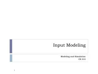
Princess Nora University. Modeling and Simulation Input Modeling and Goodness-of-fit tests. Arwa Ibrahim Ahmed. Input models. Input models provide the driving force for a simulation model. • The quality of the output is no better than the quality of inputs. steps of input model development:

E N D
Princess Nora University Modeling and SimulationInput ModelingandGoodness-of-fit tests Arwa Ibrahim Ahmed
Input models Input models provide the driving force for a simulation model. • The quality of the output is no better than the quality of inputs. steps of input model development: • Collect data from the real system. • Identify a probability distribution to represent the input process. • Choose parameters for the distribution. • Evaluate the chosen distribution and parameters for goodness of fit.
DATA COLLECTION One of the biggest tasks in solving a real problem. GIGO –garbage-in-garbage out. Suggestions that may enhance and facilitate data collection: • Plan ahead: begin by a practice or pre-observing session, watch for unusual Circumstances. • Analyze the data as it is being collected: check adequacy. • Combine homogeneous data sets, e.g. successive time periods, during the same time period on successive days. • Be aware of data censoring: the quantity is not observed in its entirety, danger of leaving out long process times. • Check for relationship between variables, e.g. build scatter diagram. • Check for autocorrelation. • Collect input data, not performance data.
IDENTIFYING THE DISTRIBUTION • Histograms • Selecting families of distribution • Parameter estimation • Goodness-of-fit tests • Fitting a non-stationary process
HISTOGRAMS [IDENTIFYING THE DISTRIBUTION] • A frequency distribution or histogram is useful in determining the shape of a Distribution. The number of class intervals depends on: • The number of observations. • The dispersion of the data. • For continuous data: • Corresponds to the probability density function of a theoretical • distribution • For discrete data: • Corresponds to the probability mass function. • If few data points are available: combine adjacent cells to eliminate the ragged appearance of the histogram.
IDENTIFYING THE DISTRIBUTION A family of distributions is selected based on: • The context of the input variable: • Shape of the histogram • Frequently encountered distributions: • Easier to analyze: exponential, normal and Poisson • Harder to analyze: beta, gamma and Weibull
IDENTIFYING THE DISTRIBUTION Use the physical basis of the distribution as a guide, for example: • Binomial: of successes in n trials. • Poisson: of independent events that occur in a fixed amount of time or Space. • Normal: disn’t of a process that is the sum of a number of component processes.
IDENTIFYING THE DISTRIBUTION • Exponential: time between independent events, or a process time that is memory less. • Weibull: time to failure for components. • Discrete or continuous uniform: models complete uncertainty. • Triangular: a process for which only the minimum, most likely, and maximum values are known. • Empirical: resample's from the actual data collected
Poisson distribution • is a discrete probability distribution that expresses the probability of a given number of events occurring in a fixed interval of time and/or space if these events occur with a known average rate and independently of the time since the last event. • Example: • Suppose you typically get 4 pieces of mail per day. That becomes your expectation, but there will be a certain spread: sometimes a little more, sometimes a little less, once in a while nothing at all. • Given only the average rate, for a certain period of observation (pieces of mail per day), the Poisson Distribution will tell you how likely it is that you will get 3, or 5, or 11, or any other number, during one period of observation.
Poisson distribution: The distribution equation If the expected number of occurrences in a given interval is λ, then the probability that there are exactly k occurrences (k being a non-negative integer, k = 0, 1, 2, ...) is equal to: Where: * e is the base of the natural logarithm (e = 2.71828...) * k is the number of occurrences of an event— the probability of which is given by the function (The random number) * k! is the factorial of k * λ is a positive real number, equal to the expected number of occurrences during the given interval. (an average rate of value.) For instance, if the events occur on average 4 times per minute, and one is interested in the probability of an event occurring k times in a 10 minute interval, one would use a Poisson distribution as the model with λ = 10×4 = 40.
Poisson distribution: Example: Consider, in an office 2 customers arrived today. Calculate the possibilities for exactly 3 customers to be arrived on tomorrow. Step1: Find e-λ. where, λ=2 and e=2.718 e-λ = (2.718)-2 = 0.135. Step2: Find λx. where, λ=2 and x=3. λx = 23 = 8. Step3: Find f(x). f(x) = e-λλx / x! f(3) = (0.135)(8) / 3! = 0.18. Hence there are 18% possibilities for 3 customers to be arrived on tomorrow.
Exponential distribution • is a family of continuous probability distributions. It describes the time between events in a Poisson process, i.e. a process in which events occur continuously and independently at a constant average rate. It is the continuous analogue of the geometric distribution. • The probability density function (pdf) of an exponential distribution is • λ is the parameter of the distribution, x is the random variable.
Exponential distribution • For example, • the rate of incoming phone calls differs according to the time of day. But if we focus on a time interval during which the rate is roughly constant, such as from 2 to 4 p.m. • during work days, the exponential distribution can be used as a good approximate model for the time until the next phone call arrives.
Binomial Distribution Definition: • The Binomial Distribution is one of the discrete probability distribution. It is used when there are exactly two mutually exclusive outcomes of a trial. These outcomes are appropriately labeled Success and Failure. • The Binomial Distribution is used to obtain the probability of observing r successes in n trials, with the probability of success on a single trial denoted by p. • Function: P(X = r) = nCr p r (1-p)n-r • where, n = Number of events r = Number of successful events. p = Probability of success on a single trial. nCr = ( n! / (n-r)! ) / r! 1-p = Probability of failure
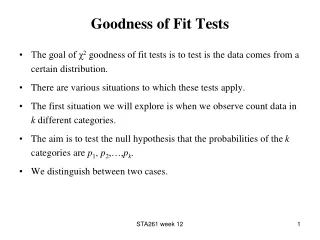
Goodness-of-fit Conduct hypothesis testing on input data distribution using: • Kolmogorov-Smirnov test • Chi-square test Goodness-of-fit tests provide helpful guidance for evaluating the suitability of a potential input model. No single correct distribution in a real application exists. • If very little data are available, it is unlikely to reject any candidate distributions • If a lot of data are available, it is likely to reject all candidate distributions.
Goodness-of-fit Intuition: comparing the histogram of the data to the shape of the candidate density or mass function Valid for large sample sizes when parameters are estimated by maximum likelihood By arranging the n observations into a set of k class intervals or cells, the test statistics is: which approximately follows the chi-square distribution with k-s-1 degrees of freedom, where s = # of parameters of the hypothesized distribution estimated by the sample statistics.
Goodness-of-fit • The hypothesis of a chi-square test is: H0: The random variable, X, conforms to the distributional assumption with the parameter(s) given by the estimate(s). H1: The random variable X does not conform. • If the distribution tested is discrete and if combining adjacent cell is not required (so that Ei > minimum requirement): • Each value of the random variable should be a class interval, unless combining is necessary, and
Goodness-of-fit If the distribution tested is continuous: where ai-1 and ai are the endpoints of the ith class interval and f(x) is the assumed pdf, F(x) is the assumed cdf. • Recommended number of class intervals (k): • Caution: Different grouping of data (i.e., k) can affect the hypothesis testing result.
Goodness-of-fit The pmf for the Poisson distribution was given: ì(e-a ax) / x! , x = 0, 1, 2 ... p(x) = í î0 , otherwise For a = 3.64, the probabilities associated with various values of x are obtained using above equation with the following results. p(0) = 0.026 p(3) = 0.211 p(6) = 0.085 p(9) = 0.008 p(1) = 0.096 p(4) = 0.192 p(7) = 0.044 p(10) = 0.003 p(2) = 0.174 p(5) = 0.140 p(8) = 0.020 p(11) = 0.001
Goodness-of-fit Vehicle Arrival Example (continued): H0: the random variable is Poisson distributed. H1: the random variable is not Poisson distributed. • Degree of freedom is k-s-1 = 7-1-1 = 5, hence, the hypothesis is rejected at the 0.05 level of significance.
Goodness-of-fit p-value for the test statistics The significance level at which one would just rejectH0 for the given test statistic value. A measure of fit, the larger the better Large p-value: good fit Small p-value: poor fit Vehicle Arrival Example (cont.): H0: data is Possion Test statistics: , with 5 degrees of freedom p-value = 0.00004, meaning we would reject H0 with 0.00004 significance level, hence Poisson is a poor fit.
Goodness-of-fit • Many software use p-value as the ranking measure to automatically determine the “best fit”. Things to be cautious about: • Software may not know about the physical basis of the data, distribution families it suggests may be inappropriate. • Close conformance to the data does not always lead to the most appropriate input model. • p-value does not say much about where the lack of fit occurs • Recommended: always inspect the automatic selection using graphical methods.
Goodness-of-fit • Fitting a NSPP to arrival data is difficult, the most practical approach: • Approximate constant arrival rate over some basic interval of time, but vary it from time interval to time interval. • Suppose we need to model arrivals over time [0,T], our approach is the most appropriate when we can: • Observe the time period repeatedly and • Count arrivals / record arrival times.
Goodness-of-fit • The estimated arrival rate during the ith time period is: where n = # of observation periods, Dt = time interval length Cij = # of arrivals during the ith time interval on the jth observation period
Goodness-of-fit • If data is not available, some possible sources to obtain information about the process are: • Engineering data: often product or process has performance ratings provided by the manufacturer or company rules specify time or production standards. • Expert option: people who are experienced with the process or similar processes, often, they can provide optimistic, pessimistic and most-likely times, and they may know the variability as well. • Physical or conventional limitations: physical limits on performance, limits or bounds that narrow the range of the input process. • The nature of the process. • The uniform, triangular, and beta distributions are often used as input models.
Goodness-of-fit • Example: Production planning simulation. • Input of sales volume of various products is required, salesperson of product XYZ says that: • No fewer than 1,000 units and no more than 5,000 units will be sold. • Given her experience, she believes there is a 90% chance of selling more than 2,000 units, a 25% chance of selling more than 3000 units, and only a 1% chance of selling more than 4,000 units. • Translating these information into a cumulative probability of being less than or equal to those goals for simulation input: