Download
1 / 1
20 likes | 249 Views
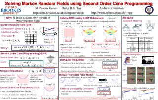
Solving Markov Random Fields using Second Order Cone Programming. Aim: To obtain accurate MAP estimate of Markov Random Fields. Results. Solving MRFs using SOCP Relaxations. Choice of S. Subgraph Matching. Desirable to eliminate Y (which squares #variables) by using slack variables.

E N D
Solving Markov Random Fields using Second Order Cone Programming Aim:To obtain accurate MAP estimate of Markov Random Fields Results Solving MRFs using SOCP Relaxations Choice of S Subgraph Matching • Desirable to eliminate Y (which squares #variables) by using slack variables. • Let ei =[ 0 0 0 … 1 … 0 0 0 ]T Markov Random Field (MRF) S = (ei + ej) (ei + ej) T S = eieiT S = (ei - ej) (ei - ej) T 1 2 3 [ 1, -1 ; -1, 1] Configuration Vector y 4 G2 = (V2,E2) G1 = (V1,E1) MRF 5 7 [ 5, 2 ; 7, 1] Likelihood Vector l • 1000 synthetic pairs of graphs • 5% noise added Prior Matrix P MRF Example #sites S = 2 #labels L = 2 Let AB = ∑ Aij Bij yi2 1 (yi + yj)2 tij (yi - yj)2 zij y* = arg min yT (4l + 2P1) - ∑ijPij zij • Objective function arg min yT (4l + 2P1) + P Y, Y = yyT subject to ∑ y(site i) = 2 - L tij + zij = 4 • Bound on slack variables tij and zij MAP y* Advantages ( A ) • Converge is guaranteed. • No restrictions on the MRF. Second Order Cone Programming (SOCP) Object Recognition • Fewer variables, faster than SDP. • Efficient interior-point algorithms. Outline Second Order Cone || u || t OR ||u||2 st Triangular Inequalities Additional constraints for better accuracy. Texture min yT f subject to || Aiy + bi || yTci + di SOCP • At least two of yi, yj and yk have the same sign. Yij + Yjk + Yik -1 Part likelihood Spatial Prior x2 + y2 = z2 • Constraints can be specified without using Y. zij + zjk + zik 8 LBP ( B ) yTq + QY, Y = yyT Convex Relaxations • Random subset of inequalities used for efficiency. Robust Truncated Prior Model Truncated for incompatible labels. GBP Semidefinite (SDP) Lift and Project (LP) • By changing values of prior, P can be made sparse. • Max-k-cut • MAP - accurate • Complexity - high • TRW-S, -expansion • MAP - inaccurate • Complexity - low SOCP Reparametrization Y - y yT 0 Y [-1,1]nxn RTPM Examples Prior [0.5 0.5 0.3 0.3 0.5] Prior [0 0 -0.2 -0.2 0] Second Order Cone Programming (SOCP) ROC Curves for 450 +ve and 2400 -ve images Additional Compatibility Constraints P(y*i,y*j) < 0 • More efficient and less accurate than SDP. • Labels for sites i and j should be compatible ∑ij P(yi,yj) zij > 0 • Relaxation • S is a set of semidefinite matrices. S = U UT S ( C ) • Choice of S is crucial for accuracy and efficiency. YS - ||UTy||2 0 Code available at http://cms.brookes.ac.uk/staff/PawanMudigonda/MRFSOCP.zip