Download
1 / 15
150 likes | 293 Views
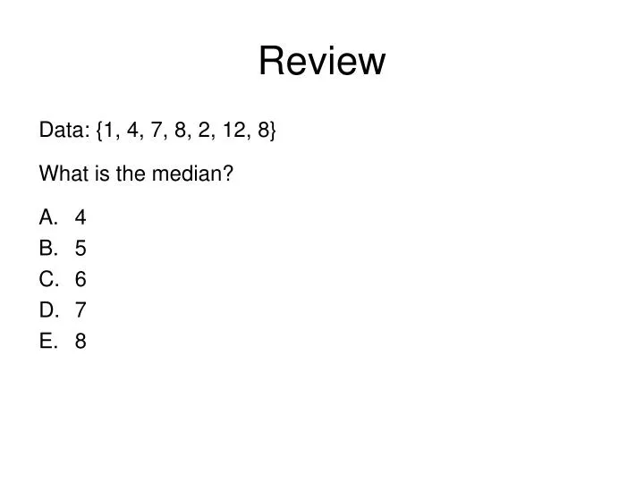
Review. Data: {1, 4, 7, 8, 2, 12, 8} What is the median? 4 5 6 7 8. Review. What scale type is this variable? Number of lever presses in a 5-min session Nominal Ordinal Interval Ratio. Review. What scale type is this variable? Points along Folsom St. between Valmont and Iris

E N D
Review Data: {1, 4, 7, 8, 2, 12, 8} What is the median? • 4 • 5 • 6 • 7 • 8
Review What scale type is this variable? Number of lever presses in a 5-min session • Nominal • Ordinal • Interval • Ratio
Review What scale type is this variable? Points along Folsom St. between Valmont and Iris • Nominal • Ordinal • Interval • Ratio
Variability 9/11
Variability • Central tendency locates middle of distribution • How are scores distributed around that point? • Low variability vs. high variability • Ways to measure variability • Range • Interquartile range • Sum of squares • Variance • Standard deviation
61 97 31 105 105 97 97 104 97 55 55 31 31 52 52 52 13 13 13 43 43 43 100 100 108 108 108 108 99 99 97 106 106 106 104 104 106 106 106 49 49 49 58 58 58 100 100 100 61 61 97 55 100 100 100 105 100 108 108 99 178 178 94 181 109 46 105 104 104 178 154 154 154 136 136 136 103 103 103 94 94 181 181 91 91 91 109 109 46 46 28 28 28 93 93 93 108 108 108 96 96 96 105 105 104 104 109 109 109 93 93 93 97 97 97 100 100 100 104 104 175 175 99 99 92 103 103 34 34 34 175 37 37 37 139 139 139 106 106 106 19 19 19 184 184 184 88 88 88 112 112 112 64 64 64 99 96 96 96 105 105 105 95 95 95 93 93 93 92 92 100 100 100 103 103 103 103 97 97 97 22 16 85 130 67 108 99 94 76 76 76 172 172 172 157 157 157 22 22 16 16 85 85 142 142 142 130 130 151 151 151 67 67 102 102 102 92 92 92 94 94 94 96 96 96 108 108 98 98 98 99 99 101 101 101 106 106 106 94 94 124 124 124 127 169 95 95 93 101 92 121 121 121 160 160 160 40 40 40 145 145 145 127 127 100 100 100 82 82 82 133 133 133 169 169 95 102 102 102 94 94 94 93 93 99 99 99 101 101 102 102 102 107 107 107 92 92 97 97 97 148 25 73 96 101 102 166 166 166 163 163 163 118 118 118 148 148 79 79 79 25 25 115 115 115 73 73 187 187 187 70 70 70 105 105 105 95 95 95 96 96 107 107 107 101 101 107 107 107 92 92 92 102 102 103 103 103 98 98 98 Average = 111.63 Average = 87.25 Average = 121 Average = 100.5 Average = 99.13 Average = 99.5 Why Variability is Important • Inference • Reliability of estimators • For its own sake • Consistency (manufacturing, sports, etc.) • Diversity (attitudes, strategies) m = 100 M 87.3 121 111.6 M 99.1 100.5 99.5
(11 – 1) + 1 = 11 Range • Distance from minimum to maximum • Sample range depends on n • More useful as population parameter • Theoretical property of measurement variable • E.g. memory test: min and max possible • Rough guidelines, e.g. height Measurement unit or precision X = [66.2, 78.6, 69.6, 65.3, 62.7] 78.6 – 62.7 + .1 = 16.0 78.65 – 62.65 = 16.0
Interquartile range • Quartiles • Values of X based on dividing data into quarters • 1st quartile: greater than 1/4 of data • 3rd quartile: greater than 3/4 of data • 2nd quartile = median • Interquartile range • Difference between 1st and 3rd quartiles • Like range, but for middle half of distribution • Not sensitive to n more stable 6 – 3 = 3 X = [1,1,2,2,2,3,3,4,4,4,4,5,5,5,5,6,6,6,6,6,7,7,7,8] 1st quartile = 3 3rd quartile = 6
m 115 88 94 108 122 133 145 Sum of Squares • Based on deviation of each datum from the mean: (X – m) • Square each deviation and add them up 729 = 272 441 = 212 49 = 72 27 21 7 7 18 30 2 = 49 2 = 324 2 = 900
m 115 88 94 108 122 133 145 Variance • Most sophisticated statistic for variability • Sum of squares divided by N • Mean Square: average squared deviation 729 = 272 441 = 212 49 = 72 27 21 7 7 18 30 2 = 49 2 = 324 2 = 900
Square Square-root Average (X – m)2 = [0, 4, 4, 1, 1, 1, 9, 4, 1, 9, 4, 0] Standard deviation • Typical difference between X and m • Again, based on (X – m)2 • Variance is average squared deviation,so sqrt(variance) is standard deviation X = [5, 3, 7, 6, 4, 6, 8, 7, 4, 2, 3, 5] m = 5 Average X – m = [0, -2, 2, 1, -1, 1, 3, 2, -1, -3, -2, 0]
Why squared difference? • Could use absolute distances, |X - µ| • Would be more intuitive: average distance from the mean • Squares have special mathematical properties • Can be broken into different parts Sum of Squares: Differences among scores Central Tendency: Common to all scores
Review Ask people how many hats they own. Data: {6, 4, 7, 8, 2, 12, 8} What is the range? • 2 • 7 • 10 • 11 • 12
Review Find the sum of squares of {6, 4, 7, 8, 2, 9}. Hint: M = 6 • 34 • 250 • 12 • 214 • 234
Review A population has a sum of squares of 6400 and a variance of 16. How big is the population (N)? • 5 • 20 • 400 • 1600 • Not enough information