Download
1 / 88
890 likes | 1.17k Views
Configuring EIGRP. Andrei Bot. April 5 th , 2012. Introduction to EIGRP Concepts EIGRP Basic configuration EIGRP traffic engineering EIGRP filtering. EIGRP concepts. Introduction

E N D
Configuring EIGRP Andrei Bot April 5th, 2012
Introduction to EIGRP Concepts EIGRP Basic configuration EIGRP traffic engineering EIGRP filtering
Introduction First released in IOS 9.21, EIGRP(Enhanced Interior Gateway Routing Protocol) is as the name says, an enhancement of the Cisco IGRP(Interior Gateway Routing Protocol) Unlike RIP and RIPv2, EIGRP is far more then IGRP with some added extensions. Like IGRP, EIGRP is a distance vector protocol and uses the same composite metrics as IGRP uses. Beyond that, there are few similarities. IGRP was removed as of IOS releases 12.2(13)T IGRP Cisco developed IGRP in the mid-1980 as an answer to the limitations of RIP but still sharing many operational characteristics with RIP: Its still a classful distance vector protocol that periodically broadcast its entire routing table(with the exception of routes suppressed by split horizon) to all its neighbors, convergence based on timers, etc. The most significant changes brought by IGRP were the hop count metric and the 15-hop network size, which carries over into EIGRP. IGRP Metrics IGRP calculates a composite metric from a variety of route variables (bandwidth, delay, load, reliability). Although hop count is not one of these variables, IGRP did track hop count and could be implemented on networks of up to 255 hops in diameter. Although the composite metric can use 4 variables, by default IGRP use bandwidth and delay only.
All variables used by IGRP in building the composite metric are visible via “show interface”. Bandwidth value is the inverse of the bandwidth scaled by a factor of which make the value in out example It is important to mention that serial interfaces on Cisco routers have a default bandwidth value of 1544 no matter what the bandwidth is of the connected link, therefore we can use bandwidth command to adjust it to the correct value. Delay value is displayed as DLY in units of microseconds and can be changed with the delay command, which specifies the delay in tens of microseconds. In our example delay value calculated by IGRP will be, us
Reliability and load are measured dynamically. For reliability 255 is 100% reliable link and 1 is a minimally reliable link, for example 234/255 or 91.8%. For load, 1 is minimally loaded link and 255 is a 100% loaded link, for example 40/255 or 15.7% load
The composite metric for each IGRP route is calculated as follows: • Where, • = minimum BW of all the outgoing interfaces along the route to the destination • = total DLY of the route • The values K1 through K5 are configurable and their default values are k1=k3=1 and k2=k4=k5=0. When k5 is set to zero [k5/RELIABILITY+k4] term is not used which reduce to the default metric:
The routing table itself shows only the derived metric but the actual IGRP metric for 172.20.40.0/24 is calculated as follows. Minimum bandwidth of the route from Casablanca to 172.20.40.0/24 is 512K at Quebec. The total delay of the route is 1000+20000+20000+5000 = 46000 microseconds
The actual IGRP values for delay and bandwidth can be seen in the “show ip route <route> It is important to note that all metrics are calculated from an outgoing interface perspective along the route. For example, the metric for the route from Yalta to subnet 172.20.4.0/24 is different from the metric for the route from Casablanca to subnet 172.20.40.0/24 IGRP Process Domains IGRP also uses the concept of process domains, allowing to isolate communications within one domain from communicating with another domain. Traffic between domains can be regulated by redistribution and filtering, allowing a more granular control over routing updates inside the routing domain.
Within AS10, there are two IGRP domains: IGRP 20 and IGRP 30. Even though 20 and 30 are defined in configuration as autonomous system numbers, in this context, the numbers serve to distinguish two routing processes within the same routing domain. Redistribution between IGRP domains is done automatically With concept of different IGRP domains, different route types are introduced. Within its update, IGRP classifies route entries into one of three categories: interior routes, system routes and exterior routes
Some other significant advantages introduced by IGRP over RIP are: *Unequal-cost load sharing *Update period 90sec three time longer then RIP’s reducing the amount of update transmitted(however, extend the convergence time) [invalid timer is set to 270/flush timer set for 630] The biggest disadvantage of both IGRP and EIGRP is that they are proprietary to Cisco and therefore limited to Cisco products.
From IGRP to EIGRP • The original motivation for developing EIGRP was simply to make IGRP classless. The result was a protocol that, while retaining some concepts introduced with IGRP such as composite metric, protocol domains and unequal-cost load balancing, is distinctly different from IGRP. • EIGRP is occasionally described as an advanced distance vector protocol • Distance Vector protocols = shares everything it knows, but only with directly connected neighbors • Link-States protocols = announce information only about their directly connected links, but they share the information with all routers in their routing domain(area) • All the distance vector protocols run some variant of Bellman-Ford algorithm. These are prone to routing loops. As a result, they must implement a loop-avoidance measures such as split horizon, route poisoning and hold-down timers, which might impact severely convergence time in a large scale network.
In contrast to Bellman-Ford algorithms used by most other distance vector protocols, EIGRP uses DUAL algorithm which ensure a fast convergence while remaining a loop-free. EIGRP packets can be authenticated using MD5 Finally, a major feature of EIGRP is that it can route not only IP but also IPX or AppleTalk.
EIGRP Packet Formats The IP header of an EIGRP packet specifies protocol number 88. Following the IP header is an EIGRP header followed by various Type/Length/Value(TLV) triplets http://www.iana.org/assignments/protocol-numbers/protocol-numbers.xml
General TLV Fields This TLVs carry EIGRP management information and are not specific to any routed protocol. IP Specific TLVs The internal and external routes TLVs include metric information for the route. The metrics used by EIGRP are the same metrics used by IGRP, although scaled by 256
Operation of EIGRP EIGRP uses the same formula that IGRP uses to calculate its composite metric. However, EIGRP scales the metric components by 256 to achieve a finer metric granularity. EIGRP has four fundamental components: 1. Protocol-Dependent Module 2. Reliable Transport Protocol(RTP) 3. Neighbor Discovery/Recovery 4. Diffusing Update Algorithm(DUAL) = 6177536
Reliable Transport Protocol(RTP) EIGRP have its own transport protocol, RTP(Reliable Transport Protocol) which manage a reliable delivery and reception of EIGRP packets. Guaranteed delivery is accomplished by using a reliable multicast, 224.0.0.10. Each neighbor receiving a reliable multicast packet unicast an acknowledgement. Ordered delivery is ensured by including two sequence numbers in the packet(sender’s sequence number and last seq. number received from the neighbor) There are multiple packet types, all of which are identified by protocol number 88 in the IP header: a). Hellos b). Acknowledgements(ACKs) c). Updates d). Queries and Replies If any packet is reliably multicast and an ACK is not received from a neighbor, the packet will be retransmitted as a unicast to that un-responding neighbor. If an ACK is not received after 16 of these retransmissions, the neighbor will be declared dead.
We can see as follows how an update is received by R1 from R2 and acknowledged
Neighbor Discovery/Recovery In the Hello packet received from a neighbor a hold time value will be included, which will tell the router he maximum time it should wait to receive subsequent hellos. If the hold timer expires before a hello is received, the neighbor is declared unreachable and DUAL is informed of the loss of a neighbor By default , the hold time is three times the Hello interval. The default can be changed on a per interface basis.
The reason behind this behavior is an ACL on R2 who drops EIGRP inbound packets R2 is sending hello messages but never receives any from R1 which results in R1 ONLY, forming a “ non-functional neighbor relation”
As soon as the existing ACL is removed, the neighbor relation is formed and routers exchanged routing updates.
Diffusing Update Algorithm(DUAL) A typical distance vector when computing the best path to a destination saves the best distance(total metric or distance as hop count) and the vector(the next hop) discarding any other available path. With EIGRP, upon startup, a router uses Hellos to discover neighbors and to identify itself to neighbors. Once a neighbor is discovered, EIGRP will attempt to form an adjacency(a logical association between two neighbors over which route information is exchanged) with that neighbor(K values must match in order for an adjacency to form) As opposed to a typical distance vector, EIGRP builds a topology table based on its neighbor’s advertisements(rather than discarding the data) and converges by either looking for a likely loop-free route in the topology table or if it knows of no other route, by querying its neighbors.
Feasible Distance(FD) is the best metric along a path to a destination network, including the metric to the neighbor advertising that path Advertised Distance(AD) is the total metric along a path to a destination network as advertised by an upstream neighbor Feasible Successor(FS) is a path whose reported distance is less than the FD(current best path), Feasibility Condition. via four: AD: (10^7/10000+200)*256 = 307200 FD: (10^7/56+2200)*256 = 46277376 via three: AD: (10^7/10000+200)*256 = 307200 FD: (10^7/128+1200)*256 = 20307200 FD: 20307200, Successor router: three FS: router four???
From router one perspective: via four [FD/AD]: 20307200/307200 via two [FD/AD]: 46789376/46277376 FD:(10^7/128+1200)*256 = 20307200 FD:(10^7/56+4200)*256 = 46789376 AD:(10^7/10000 +200)*256 = 307200 AD:(10^7/56+2200)*256 = 46277376 Successor, router four, No Feasible Successor If the link to router four goes down, One will have no feasible successor towards Network a, therefore it will start to query its neighbors(router two) for a path to Network a. Router two has installed the path via router three(FD:46277376) therefore will reply to query received from router One, resulting in a new path towards Network a from router one perspective, via router two.
Prefix-lists Prefix-lists are used to match on prefix and prefix-length pairs. Normal prefix-list syntax is as follows: Where, “w.x.y.z“ is your exact prefix and “len” is your exact prefix-length ip prefix-list LIST permit 1.2.3.0/24 would be an exact match for the prefix 1.2.3.0 with a subnet mask of 255.255.255.0. When you add the keywords “ge” or “le” to the prefix-list, the “len” value change its meaning. When using GE and LE, the “len” value specifies how many bits of the prefix you are checking, starting the most significant bit. check the first 24 bits of the prefix 1.2.3.0. The subnet mask be less than equal to 32 This match everything This match a default route In many situations a prefix-list can be replaced with an access-list, however there might be scenarios where an ACL does not match the exact prefix
On R2 we cannot filter 10.0.0.0/24 by using an ACL without filtering also the summary address coming from R1, 10.0.0.0/22 10.0.0.0 255.255.255.0 – will match first 24 bits, however first 22 will match the same bits from our summary address. By using following ACL, access-list 1 deny 10.0.0.0 0.0.0.255 we drop 10.0.0.0/24 and 10.0.0.0/22
Using a prefix-list we can deny the /24 prefix while /22 will be permited
Route Maps Route maps is a powerful tool for creating customized routing policies. They are similar to ALC, both having criteria for matching the details of certain packets and an action of permitting or denying those packets. Unlike access-lists, route maps can add to each “match” criteria a “set” criteria that actually changes the packet in a specific manner Each route map statement has a “permit” or “deny” action and a sequence number. At the end, an implicit deny exist as for ACLs. A packet or route is passed sequentially through route-map statement . If a match is made, any set statement are executed and the permit or deny action is executed. As with ACLs, processing stops when a match is made and the specific action is executed. The route or packet is not passed to subsequent statements.
Network statement The network statement control what interfaces are running the EIGRP process. By using a wildcard mask we can be more specific in identifying an interface(s)
EIGRP Auto-summary EIGRP was built as a classless protocol, however, by default still have a classful behavior to facilitate interaction with IGRP. With auto-summarization enabled by default, networks are summarized as they pass through the major network boundary.
Having auto-summary on, will prevent advertisement of discontiguous networks. With EIGRP auto-summary disabled the subnets of the discontiguous network 120.1.0.0/16 can be advertised.
EIGRP Topology table Once the adjacency is established, every EIGRP router is building it’s own topology table.
By showing a specific entry in the topology table, we can see the entire vector metric
EIGRP equal cost load balancing By default EIGRP load balance traffic over 4 equal paths(with the same metric) By altering values of delay or bandwidth we can get equal metrics towards a destination resulting in load balancing traffic over multiple paths
By default, load balancing is done on a per-destination which will not imply an equal distribution of traffic over the used links. We can see by sending 2 packets of ICMP traffic, both have as an outbound interface s0/0(125.1.12.1)
By disabling IP CEF we are getting a packet switching forwarding type of traffic, resulting in per packet load balancing and a more visible traffic share between links.
EIGRP unequal load balancing By default EIGRP uses bandwidth and delay to calculate its composite metric. Load and reliability can also be used, or the ratio at which bandwidth and delay are used can be changed by modifying the metric weights. The default weighting of K1 =1 and K3 = 1 means that only bandwidth and delay are used.
show ipeigrp topology show the individual vector metrics that are used in the composite calculation Trying to engineer traffic in a more complex network can get in very complicated calculations using both values, therefore we can select to have only the value(s) that we consider useful or required in our specific scenario. A very important thing to remember is that K values must match on both sides, otherwise an adjacency will not be formed.