Download
1 / 41
420 likes | 672 Views
1. A Brief History of Risk and Return. A Brief History of Risk and Return. Two key observations: There is a substantial reward, on average, for bearing risk. Greater risks accompany greater returns. Dollar & Percent Returns.

E N D
1 A Brief History of Risk and Return
A Brief History of Risk and Return • Two key observations: • There is a substantial reward, on average, for bearing risk. • Greater risks accompany greater returns.
Dollar & Percent Returns • Total dollar return= the return on an investment measured in dollars • $ return = dividends + capital gains • Total percent returnis the return on an investment measured as a percentage of the original investment. • % Return = $ return/$ invested • The total percent return is the return for each dollar invested.
Percent Return Dividend Yield Capital Gains Yield
Example: Calculating Total Dollar and Total Percent Returns • You invest in a stock with a share price of $25. • After one year, the stock price per share is $35. • Each share paid a $2 dividend. • What was your total return?
Annualized Returns Effective Annual Rate (EAR) Where: HPR = Holding Period Return M = Number of Holding Periods per year
Annualized Returns – Example 1 You buy a stock for $20 per share on January 1. Four months later you sell for $22 per share. No dividend has been paid yet this year. P0 = $20 P.33 = $22 t =“.33” since 4 months is 1/3 of a year 4-month HPR = 3 periods per year Holding Period Return (HPR) Annualized Return (EAR)
Annualized Returns – Example 2 Suppose the $20 stock you bought on January 1 is selling for $28 two years later No dividends were paid in either year. P0 = $20 P2 = $28 HPR = 2 years (t = 2) HPR per year = ½ (0.50) Holding Period Return (HPR) Annualized Return (EAR)
The Historical Record: Total Returns on Small-Company Stocks
Historical Average Returns • Historical Average Return = simple, or arithmetic average. • Using the data in Table 1.1: • Sum the returns for large-company stocks from 1926 through 2006, you get about 984 percent. • Divide by the number of years (80) = 12.3%. • Your best guess about the size of the return for a year selected at random is 12.3%.
Average Returns: The First Lesson • Risk-free rate: • Rate of return on a riskless investment • Risk premium: • Extra return on a risky asset over the risk-free rate • Reward for bearing risk • The First Lesson:There is a reward, on average, for bearing risk.
Risk Premiums • Risk is measured by the dispersion or spread of returns • Risk metrics: • Variance • Standard deviation • The Second Lesson:The greater the potential reward, the greater the risk.
Return Variability Review and Concepts • Variance(σ2) • Common measure of return dispersion • Also call variability • Standard deviation(σ) • Square root of the variance • Sometimes called volatility • Same "units" as the average
Return Variability:The Statistical Tools for HistoricalReturns • Return variance: (“N" =number of returns): • Standard Deviation
Example: Calculating Historical Variance and Standard Deviation • Using data from Table 1.1 for large-company stocks:
Return Variability Review and Concepts • Normal distribution: • A symmetric, bell-shaped frequency distribution (the bell-shaped curve) • Completely described with an average and a standard deviation (mean and variance) • Does a normal distribution describe asset returns?
Frequency Distribution of Returns on Common Stocks, 1926—2006
Historical Returns, StandardDeviations, and Frequency Distributions: 1926—2006 1-26
The Normal Distribution and Large Company Stock Returns 1-27
Arithmetic Averages versusGeometric Averages • The arithmetic average return answers the question: “What was your return in an average year over a particular period?” • The geometric average return answers the question: “What was your average compound return per year over a particular period?”
Geometric Average Return: Formula Equation 1.5 Where: Ri = return in each period N = number of periods
Geometric Average Return Where: Π= Product (like Σ for sum) N = Number of periods in sample Ri = Actual return in each period
Example: Calculating a Geometric Average Return • Using the large-company stock data from Table 1.1:
Arithmetic Averages versusGeometric Averages • The arithmetic average tells you what you earned in a typical year. • The geometric average tells you what you actually earned per year on average, compounded annually. • “Average returns” generally means arithmetic average returns.
For forecasting future returns: Arithmetic average "too high" for long forecasts Geometric average "too low" for short forecasts Geometric versus Arithmetic Averages
Blume’s Formula • Form a “T” year average return forecast from arithmetic and geometric averages covering “N” years, N>T.
Check This 1.5aCompute the Average Returns Arithmetic Average Geometric Average
Risk and Return • The risk-free rate represents compensation for the time value of money. • First Lesson: • If we are willing to bear risk, then we can expect to earn a risk premium, at least on average. • Second Lesson: • The more risk we are willing to bear, the greater the expected risk premium.
Chapter 1 End A Brief History of Risk and Return