Download
1 / 15
150 likes | 250 Views
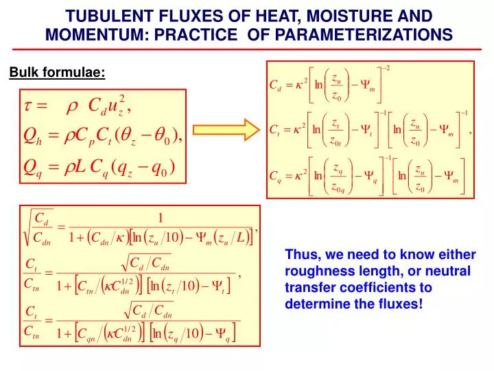
TUBULENT FLUXES OF HEAT, MOISTURE AND MOMENTUM: PRACTICE OF PARAMETERIZATIONS. Bulk formulae:. Thus, we need to know either roughness length, or neutral transfer coefficients to determine the fluxes!. C d (unstable). C dn. ~10 -3. C d (stable). V.

E N D
TUBULENT FLUXES OF HEAT, MOISTURE AND MOMENTUM: PRACTICE OF PARAMETERIZATIONS Bulk formulae: Thus, we need to know either roughness length, or neutral transfer coefficients to determine the fluxes!
Cd (unstable) Cdn ~10-3 Cd (stable) V 1. Typical approach: parameterization from measurements • To measure the flux (eddy correlation or inertial dissipation) under • the neutral conditions and the mean variables simultaneously; • To derive experimental dependence of the neutral transfer • coefficient on the wind speed; • To apply stability correction functions and to derive coefficients for • different stability conditions.
Parameterizations derived from field measurements: Garratt (1977) for the momentum flux + Garratt and Hyson (1975) for sensible and latent fluxes. About 790 eddy correlation measurements in different conditions from different platforms. Kruegermeyer (1976) – 124 hours of profile measurements in the tropics. Hasse et al. (1978) – 1400 hours of profile measurements in the Tropical Atlantic (coefficients for neutral conditions) 4. Smith and Banke (1975), Smith (1980), Smith (1988) – eddy correlation measurements with a thrust anemometer at a platform offshore US West coast. Stability correction: Bussinger et al. (1973), Dyer (1974), Paulson (1970).
Smith 88 Large and Pond (1981, 1982) – same platform as Smith (1980, 1988), eddy correlation + inertial dissipation measurements. Additionally ship measurements in the Atlantic and Pacific were used. Scatter was slightly better for the neutral coefficients for heat and moisture dependent on Cdn, than for the constant coefficients.
2. Modelling of surface atmospheric layer to determine exchange coefficients Liu, Katsaros and Bussinger (1979) (LKB) – surface renewal theory. Surface renewal theory was first introduced in chemical engineering and has been applied to air-sea interface by Liu and Bussinger (1975) and Liu et al. (1979). Main assumption: Whereas the atmospheric (and oceanic) surface boundary layer transports heat, mass and momentum to the interface by turbulent motions, at the surface itself there exists an interfacial layer of order 1 mm thick, in which molecular diffusion plays a significant role in the transport. Across this interfacial layer, small eddies of air transfer heat randomly and intermittently between the “bulk” turbulent fluid, of temperature Tb, and the surface itself which therefore warms or cools by conduction from the eddies.
The temperature gradient and the surface heat flux are determined by the heat conduction equation: Thermal diffusivity The solution for initial condition T(t=0) = Tb= constant, and surface temperature T(z=0) = Ts= constant: - heat flux Liu and Businger (1975) introduced a function to describe the areal fraction of eddies which have been in contact with the surface for time t, and assume a characteristic time, tc, for which an eddy remains in contact with the surface before breaking away. For constant Tsand a random distribution of contact duration the time-averaged temperature profile in the interfacial layer: - LKB flux-profile relationship and an average heat flux:
Values of the exchange coefficients for LKB, as functions of wind speed and stability
Variations of coefficients from different schemes • Differences in behaviour of the coeeficients with wind are in general larger than with stability, at least for moderate and strong winds • The largest uncertainty in stability is observed under small winds Typical variations: Cd, Ct, Ce ~ 0.5x10³ • Recommendations: • Do not hesitate to use simple paramterizations; • Try to rely more on parameterizations derived from field observations • Under the calm or low winds use LKB, if ……[LATER]!!!!! • Never say “The best parameterization is done by XXXX” – they are all very uncertaint • Smith (1988) is considered to be most reliable • More or less “officially recommended” are Smith (1988), Large and Pond (1981, 1982), LKB • (among these very simple parameterizaions)
“field-only” schemes universal schemes: modelling, surface renewal theory Clayson et al. (1996) Zeng et al. (1998) Beljaars (1995) Bourassa et al. (1996) ASTEX - White et al. (1995) CATCH - Eymard et al. (1998) FASTEX – Hare et al. (1995) LabSea: Bumke et al. (2002) COARE-3.0 algorithm (Fairall et al. 2003)
COARE-3.0 algorithm (Fairall et al. 2003) • Based on the TOGA-COARE results and 2777 covariance flux • measurements at the ETL; • Tested using 4439 new values from field experiments between • 1997 and 1999 including the wind speed regime beyond 10 m; • The average (mean and median) model results agreed with the • measurements to within about 5% for moisture from 0 to 20 m.
Variations in turbulent fluxes due to different parameterizations North Atlantic
/helios/u2/gulev/handout: lapo3.for - Large and Pond (1981, 1982) –with German comments liu3.for – LKB (Liu, Katsaros and Bussinger 1979) potsmin1.for - Smith (1988) (all codes are for water vapor pressure, i.e. ez and not q) Compute the fluxes of sensible heat, latent heat and momentum for the following conditions: SST=10C, Ta=8C, ez=9mb, V=7m/s, Pa=1010mb SST=10C, Ta=12C, ez=11mb, V=7m/s, Pa=1010mb SST=10C, Ta=8C, ez=9mb, V=3m/s, Pa=1010mb SST=10C, Ta=8C, ez=9mb, V=12m/s, Pa=1010mb
/helios/u2/gulev/handout/ (for the same parameter values) flux_test.f – program to compute instantaneous values of urbulent fluxes, using Liu et al. (1979), Large and pond (1981, 1982) and Simth (1988) schemes. Compilation: • f77 –o flux_test flux_test.f lapo3.for liu3.for potsmin1.for • Results: • flux.res
References Blanc, T.V., 1985: Variation of bulk-derived surface flux, stability and roughness results due to the use of different transfer coefficient schemes. J. Phys. Oceanogr., 15, 650-669. Blackadar, A., 1998: Turbulence and diffusion in th eatmosphere. Springer-Verlag, 186 pp. Blanc, T.V., 1987: Accuracy of bulk-method determined flux, stability, and sea surface roughness. J. Geophys. Res., 92, 3867-3876. Bumke, K., U.Karger, and K.Uhlig, 2002: Measurements of turbulent fluxes of momentum and sensible heat over the Labrador Sea. J.Phys. Oceanogr, 32, 401-410. da Silva, A.M., C.C. Young, and S.Levitus, 1994: Atlas of surface marine data. NOAA Atlas NESDIS 6, Volume 1-6, US Dept. Commerce, NODC, NOAA/NESDIS, Washington DC. Dyer, A.J., 1974: A review of flux-profile relationships, Bound.-Layer Meteor., 7, 363-372. Eymard, L., G. Caniaux, H.Dupuis, L.Prieur, H.Giordani, R.Troadec, P.Bessemoulin, G. Lachaud, G.Bouhours, D.Bourras, C.Guerin, P.LeBrogne, A.Brisson, and A. Marsouin, 1999: Surface fluxes in the North Atlantic current during CATCH/FASTEX. Quart. J. Roy. Meteor. Soc., 125, 3563-3599. Fairall, C. W., E. F. Bradley, D. P. Rogers, J. B. Edson, and G. S. Young, 1996: Bulk parameterization of air-sea fluxes for Tropical Ocean-Global Atmosphere Coupled-Ocean Atmosphere Response Experiment. J. Geophys. Res., 101, 3747-3764. Geernaert, G., and W.J.Plant, 1990: Surface waves and fluxes. Kluwer AP, 2 volumes. Golitsyn, G.S., and A.A.Grachov, 1986: Free convection of multi-component media and parameterization of air-sea interaction at light winds. Ocean-Air Interactions, 1, 57-78. Grachov, A.A., and G. Panin, 1984: Sensible and latent heat flux parameterization over water surface under natural conditions. Izv. Acad. Sci. USSR. Atmos. Oceanic. Phys. 20, 364-371. Hasse, L., 1971: The sea surface temperature deviation and the heat flow at the sea-air interface. Bound.-Layer Meteor., 1, 368-379. Hasse, L., and S.D. Smith, 1997: Local sea surface wind, wind stress, and sensible and latent heat fluxes. J.Climate, 10, 2711-2724. Isemer, H.-J., and L. Hasse, 1987: The Bunker Climate Atlas of the North Atlantic Ocean. Vol.2, Air-Sea Interactions, Springer-Verlag, 252 pp.
References-continue Josey, S., E.C.Kent, and P.K.Taylor, 1999: New insights into the ocean heat budget closure problem from analysis of the SOC air-sea flux climatology. J. Climate, 12, 2856-2880. The LabSea Group, 1998: The Labrador Sea Deep convection Experiment. Bull Amer. Met. Soc., 79, 2033-2058. Large, W.G., and S.Pond, 1981: Open ocean momentum flux measurements in moderate to strong winds. J. Phys. Oceanogr., 11, 324-336. Large, W.G., and S.Pond, 1982: Sensible and latent heat fluxes over the ocean. J.Phys.Oceanogr., 12, 463-482. Liu, W.T., K.Katsaros, and J.Businger, 1979: Bulk parameterization of air-sea exchanges of heat and water vapor including molecular constraints at the interface. J.Atmos.Sci., 36, 1722-1735. Oberhuber, J.M., 1988: An Atlas based on the COADS data set: the budgets of heat, buoyancy and turbulent kinetic energy at the surface of the global ocean. MPI fuer Meteorologie report, No. 15, 19pp. [Available from Max-Plank-Institute fuer Meteorologie, Bundesstrasse 55, Hamburg, Germany]. Paulson, C.A., 1970: Representation of wind speed and temperature profiles in the unstable atmospheric surface layer. J. Appl. Meteor., 9, 857-861. Renfrew, J., G.W.K. Moore, P.S. Guest and K. Bumke, 2002: A comparison of surface-layer, surface heat flux and surface momentum flux observations over the Labrador Sea with ECMWF analyses and NCEP reanalyses. J. Phys. Oceanogr., 32, 383-400 Smith, S.D., 1980: Wind stress and heat flux over the ocean in gale force winds. J. Phys. Oceanogr., 10, 709-726. Smith, S.D., 1988: Coefficients for sea surface wind stress, heat flux and wind profiles as a function of wind speed and temperature. J.Geophys. Res., 93, 15467-15474. Stull., R., An introduction to boundary layer meteorology. Kluwer AP, 667 pp. Yelland, M.J., B.I.Moat, P.K.Taylor, R.W.Pascal, J.Hutchings, and V.C.Cornell, 1998: Wind stress measurements from the open ocean corrected for air flow disturbance by the ship. J. Phys. Oceanogr., 28, 1511-1526. Zeng, X., M. Zhao, and R. Dickinson, 1998: Intercomparison of bulk aerodynamic algorithms for the computation of sea surface fluxes using TOGA COARE and TAO data. J.Climate, 11, 2628-2644.