Download
1 / 23
260 likes | 462 Views
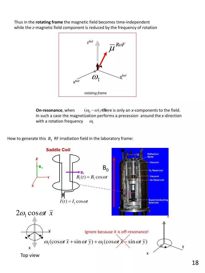
Thus in the rotating frame the magnetic field becomes time-independent while the z -magnetic field component is reduced by the frequency of rotation . z RoF. y RoF. x RoF. rotating frame. On-resonance , when , there is only an x -components to the field.

E N D
Thus in the rotating frame the magnetic field becomes time-independent while the z-magnetic field component is reduced by the frequency of rotation zRoF yRoF xRoF rotating frame On-resonance, when , there is only an x-components to the field. In such a case the magnetization performs a precession around the x-direction with a rotation frequency . How to generate this B1 RF irradiation field in the laboratory frame: B0 z y Ignore because it is off-resonance! y x x Top view 18
Bird cage National High Magnetic Field Laboratory Doty Scientific u-of-o-nmr-facility.blogspot.com/2008/03/prob... in: Thus the magnetic field in the laboratory frame : Becomes in the rotating frame: out: In NMR we measure the magnetization in the rotating frame: Although the signal detection in the laboratory frame is along the direction of the coil: A sample with an overall f =noise of apparatus h =filling factor n =frequency Dn=band width Q =quality factor Vs =sample volume the S/N voltage at the coil is: 19
2d-i complex numbers A large part of our discussion will deal with precessions of vectors, and with expressions that need complex numbers. Here we introduce these numbers and give some necessary rules. Let us suppose that there are “numbers” that in fact are composed of two numbers: These complex numbers have their own mathematics based on : imaginary axis b real axis a Im A common practice is to present the values of the x- and y-components of the magnetization as if they are one complex number: Re A precessing magnetization around the z-direction has as xy-components the value: This can be written as Im with the definition 1 Re 2d. Necessary concepts for QM description 20
There is no way of explaining NMR without some Quantum Mechanics: Here we give rules that can help us to “understand” what we are measuring in NMR. Because the spin behave according to the theory of QM, the necessary “rules” we need to proceed are: (We are all used to presenting spectroscopy by , but why? ) 1. A stationary quantum system experiencing a time independent environment (Hamiltonian) will preside in one of its discrete (constant energy) eigenstates. A spin-1/2 system, like the proton or an electron, in a magnetic field has only two eigenstateswith energies according to the z-components of their magnetization . The allowed components of the angular momentum are with . The way to present these energies is by an energy level diagram and the eigen states by : m is called the magnetic quantum number . The actual length of the angular momentum is but we can only determine its z-component. In fact we do not know what the phase of its xy- component is. When the spin is in one of these states it is stationary 2d-ii Wavefuntions, eigenstates and observables 21
In analogy, a spin-I can occupy eigenstates with energies and spin=3/2 : In general: 2. A dynamic quantum system can find itself in a linear superposition of its eigenstates. for a spin ½: 3. The result of a measurement of an observable O can be obtained by a calculation of the form knowing the value of the elements with 22
2d-iv Matrix representation define a basis set spanning Hilbert space that is orthonormal. This enables a matrix representation of any operator and a vector representation of any wave function. When the representation of an operator is diagonal, then the basis set is the eigenbasis set and the matrix elements the eigenvalues. When the representation of an operator is not diagonal then after diagonalization we obtain the eigenfunctions and eigenvalues the eigenvaluesof the Hamiltonian are the energies of the system 23
d-v The Schrodinger Equation Vector-matrix representation a time dependent Hamiltonian doesn’t have eigenvalues/energies The solution of the Schrodinger equation defines an evolution operator If the Hamiltonian is time independent then If the Hamiltonian is time dependent then, with the Dyson operator T: 24 t
d-vi. The angular momentum operators, definitions an cyclic permutation in the eigenfunction representation: 25
In the basis set of Iz: Pauli matrices span the whole2x2Hilbert space In the basis set of Iz: The linear angular momentum operators do not span the whole3x3Hilbert space The missing operators are: 26
2d-vii A nucleus in a magnetic field The spin Hamiltonian with the magnetic field in the z-direction of the lab. frame and an RF irradiation: and the rotating frame: For spin=1/2 : Pauli matrices cyclic permutations: 27
Remember that when the Hamiltonian is time independent and is Hemitian is unitary 28
2d-viii The spin-density operator An arbitrary function can be expended in a basis set This defines a set of coefficients with Let us define an operator with matrix elements Is Hermitian 29
2d-ix Ensemble Average and thermodynamics Consider an ensemble average of the matrix elements of the spin-density In the representation of the eigenbasis of the Hamiltonian the solution for the density matrix elements LNN LN-1,N-1 L22 L11 then with the random phase approximation coherences the populations 30
Thus the equilibrium density operator can be defined by the populations satisfying the Boltzman statistics In NMR we solve the Liouville-von Neumanequation: The signal is proportional to an “observable” 31
This requires a definition of the populations of the eigenstates. At thermal equilibrium these populations follow the Boltzmann distribution: and the populations become The thermal-equilibrium ensemble magnetization becomes ………….. This require a definition of the populations of the eigenstates. 32
A similar derivation can be presented for a spin higher than ½ in a magnetic field. The Boltzman distribution at high temperature results in The magnitude of at 50-300K is very small. and the bulk magnetization becomes and the populations become Despite these very small values the ensemble nuclear magnetization can be detected. The thermal-equilibrium ensemble magnetization becomes 33
2d-x NMR is a journey along the matrix elements of the reduced spin density matrix Example of pulse on I=1/2 NMR signals Coherences that are off diagonal element are detected. Populations that are the diagonal element are not detected 34
2d-xi (high temperature) NMR on S=1/2 The Larmor precession for spin I=1/2 35
NMR signals in the Rotating frame z “quadrature detection” 36 y x
A symbolic summary without explicitly calculating the reduced density matrix Define the spin system by its equilibrium density operator: The environment of the spin system is defined by the Hamiltonian: and in the rotating frame: Here the Hamiltonians H correspond to magnetic fields Bp in the p-direction According to the rotation properties of the angular moment operator The Hamiltonian “rotates” the spin density operator The density operator can be “measured” by calculating “observables” resulting here in the magnetization {Mp}
The transverse components of the bulk magnetization can only become zero when all individual spins behave the same and there is no phase-scrambling. Thus, when we manipulate the spins simultaneously in an equal manner, the bulk magnetization behaves like a single spin. Just as we described the motion of a single spin in the laboratory and rotating frame, we can present the bulk magnetization in the lab and rotating frame. z zRoF y yRoF x xRoF Laboratory frame rotating frame The bulk magnetization during an RF irradiation field. This result is like an indication that the classical motion of the magnetization for a spin-1/2 behaves like the QM result. For spin-1/2 we can use the vector picture derived before for the magnetization precession around any external magnetic field. For spins higher than ½ the number of elements of the angular momentum components becomes larger and we will have to show that these components also result in a precession motion of its classical magnetization. For further reading about QM, take any book on an “Introduction to Quantum Mechanics” 38
zRoF Slow fluctuating components, contribute to T1 yRoF xRoF Fastfluctuating components at the order of contribute to T1 and T2 2eT1 and T2 Relaxation The return of the bulk magnetization to thermal equilibrium is governed by thermal motions. We distinguish between two mechanisms, th0e dephasingof the transverse component with a typical time constant T2 and the buildup of the longitudinal component to thermal equilibrium with a time constant T1. zRoF yRoF xRoF A simplistic way of understanding the action of the T1 and T2 relaxation mechanisms is to consider thermally fluctuating magnetic fields in the laboratory frame. These fields will rotate the individual components of the magnetization and a dephasing process will decrease the magnitude of the transverse magnetization and Increase the longitudinal magnetization towards equilibrium. The interaction of the spins their thermal bath will results in a Boltzmann population of their spin levels. That there is a difference between the two relaxation times can be understood by realizing that the individual magnetizations are precessing around the external magnetic field. To influence the direction of the z-magnetizations the small fluctuating fields must be constant for a sufficient time. To influence the phases of the xy-magnetizations the fluctuating field must be have components that vary at the order of the Larmor frequency. For a randomly fluctuating field in the lab. frame . 39
During an NMR experiment the nuclei are irradiated by a linear oscillating small magnetic field: 40