Download
1 / 64
730 likes | 1.31k Views
Basics of Audio Signal Processing. Sudhir K. Digital Representation of Audio Psycho-Acoustic principles Lossy Compression of Audio (MP3 and AAC) Lossless compression of Audio (general principles with example). Summary Slide. PCM Data

E N D
Basics of Audio Signal Processing Sudhir K
Digital Representation of Audio Psycho-Acoustic principles Lossy Compression of Audio (MP3 and AAC) Lossless compression of Audio (general principles with example) Summary Slide
PCM Data Sampling audio input at discrete intervals and quantizing into discrete number of evenly spaced levels. Sampling Frequency Bits per sample Number of Channels Interleaved and block format Audio CD 44.1 KHz, 2 channels , data-rate is 1.4 Mbits per second ADC Digital Processing DAC speakers Digital Representation of Audio
Sound Pressure Level Perceptual and Statistical redundancy Absolute Threshold of Hearing Critical Bands Masking in Time domain Masking in Frequency domain Perceptual Entropy Pre-echo Effect Psycho-Acoustic Model 1 Psycho-Acoustic Model 2 Filter Banks and Transforms Psycho-Acoustic Principles
Standard metric to quantify intensity of acoustical stimulus Measured in decibels (dB) relative to an internationally defined reference level Sound Pressure Level • LSPL is the SPL of stimulus p • P0 is the standard reference level at 20 µPa • 150-dB SPL is the dynamic range of human auditory system • 140-dB SPL is typically the threshold of pain • Human auditory system can hear frequencies ranging from 20 Hz to 20 KHz frequency
Characterizes the amount of energy needed in a pure tone such that it can be detected by a listener in a noiseless environment This can be interpreted naively as a maximum allowable energy level for coding distortions introduced in frequency domain Absolute Threshold of Hearing • Note that the absolute threshold of hearing is a function of frequency • Response of a human ear for a pure tone is dependant on the frequency of the tone • Sensation Level : intensity level difference for stimultus relative to detection threshold (quantifies listener’s audibility) • Equal SL components can have different SPL’s
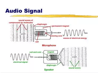
Frequency to place transformation Sound wave moves the eardrum and attached bones The eardrum and the bones transfer mechanical vibrations to Cochlea Oval window of cochlear membrane induces traveling waves along length of basilar membrane. Traveling waves generate peak responses at frequency specific membrane positions Specific positions of membrane provide peak responses for specific frequency band Cochlea can be considered as a set of highly overlapped band-pass filters. Human Ear Model
Cochlea can be considered as a set of highly overlapped band-pass filters. Critical bandwidth is a function of frequency that quantifies the cochlear bandwidth Loudness (percieved intensity) remains same when the noise energy in present within a critical band One bark corresponds to distance of one critical band Critical bandwidth tends to remain constant up to 500Hz and then increases to 20% of center frequency above 500 Hz 0 2 4 6 8 10 12 14 16 18 20 Frequency (KHz) Critical Bands
Process where one sound is rendered inaudible by presence of another sound Frequency domain masking Masker Maskee Simultaneous Masking • Tone masking Noise (TMN) • Noise Masking Tone • Noise Masking Noise • In-band Phenomenon (occurs within same critical band)
SMR (signal to mask ratio) smallest difference between intensity of masking signal and the intensity of masked signal SMR for NMN is 26dB, TMN is 24dB and NMT is 5dB Noise is a better masker than tone Spread of Masking Inter-band Masking Triangular spreading function Simultaneous Masking
Masking in time-domain Pre-Masking : Masking occurs prior to the signal Post-Masking: Masking following the occurrence of signal Pre-masking is usually less (approx 1-2 ms) Post-masking is of longer duration (50 to 300ms) Temporal (Non-simultaneous) masking
Also called as global masking threshold Global Masking threshold is a combinaton of individual masking thresholds (threshold due to NMT, TMN and absolute threshold) Quantization noise should be kept below the JND to keep it inaudible. Signal Masking curve Noise Just Noticeable Difference (JND)
Measure of perceptually relevant information Expressed in bits per sample Represents a theoretical limit on compressibility of a particular signal Perceptual Entropy
Pre-echoes occur when a signal with sharp attack begins near end of a transform block immediately following a region of low energy Pre-Echo Inverse quantization spreads evenly throughout the reconstructed block
Bit-reservoir Store surplus bits, which can be used during periods of attack Window Switching Switch between long and short time-window Short window for transients to minimize spread of noise. Long window for normal case to increase compression efficiency Gain Modification Smoothes transient peaks by changing gain of signal prior to the transient Temporal Noise Masking Linear prediction on frequency domain spectrum Flattened residual and quantization noise. The quantization noise is suchthat it follows original signal enveope Pre-Echo control
MS-Stereo (Middle/Side Stereo) One channel to encode information identical between left and right channel One channel to encode differences between left and right channel Transmit sum and difference of the original signals in left and right channels Intensity Stereo Lossy Coding technique Replace left and right channel with a single representing signal plus directional information Usually used only in higher frequencies (since human ear is less sensitive to signal phase at these frequencies) Used only at low bit-rates Stereo coding
Spectral analysis and SPL normalization Normalize input samples and segment into blocks Identification of Tonal and Noise maskers Energy from 3 adjacent spectral components combined to form single tonal masker Energy of all other spectral lines not within a range of Δ combined to form noise masker Decimation and reorganization of maskers Any tonal or noise threshold below absolute threshold are discarded Adjacent pair of maskers are compared and is replaced by stronger of the two. Calculation of individual Masking Threshold Calcullate threshold due to tonal and noise maskers Psycho Acoustic Model1
Pyscho Acoustic Model 1 Threshold due to tonal maskers Threshold due to noise maskers
Calcullation of global masking threshold Individual masking threshold are combined to estimate global masking threshold Assumes masking effects are additive Sum of absolute threshold of hearing, threshold from tonal masker and threshold from noise masker Psycho Acoustic Model 1
Lossless (analysis and synthesis should be invertible) Aliasing errors should cancel for perfect or near-perfect reconstruction Low computational complexity Bandwidth should replicate critical bands of human ear. Filter Bank Characteristics
Cosine Modulation of low-pass prototype filter to implement parallel M-channel filter banks with nearly perfect reconstruction Overall linear phase and hence constant group delay Complexity = one filter + modulation Critical sampling Pseudo-QMF Analysis & synthesis filters satisfy mirror image conditions to eliminate phase distortion Analysis filter Synthesis filter MPEG1 uses a 32-channel PQMF bank for spectral decomposition in layer I and Layer II
De-correlate signal by mapping to an orthogonal basis functions Lapped orthogonal block transform Successive transform block overlap each other Overall linear phase Forward MDCT 50% Overlap between blocks Block transform of 2M samples and block advance of M samples Basis functions extend across 2 blocks (blocking artifacts elimination) Critically sampled M samples output for 2M input samples MDCT (TDAC)
Decoded output is not bit-exact with original input Decoded output is perceptually same as original input More compression achieved Extensive use of psycho-acoustic model to discard perceptually irrelevant audio data Examples : MP3 and AAC Lossy Audio Compression techniques Time to Frequency Filter Bank Allocate bits & Quantize Format Bitstream Psycho- Acoustics Model
Audio Decoder Usually Encoder Complex and Decoder less complex
ISO 11172-3 ISO (MPEG 1) Mainly specifies the bit-stream and hence leaves the flexibility of Encoder design to individual developers Lossy and perceptually transparent Sampling frequencies of 32, 44.1 KHz and 48 KHz supported Various bit-rates from 32-192 kbps per channel supported Supports following channel modes Mono, Stereo, Dual Mono, Joint Stereo Based on complexity 3 independent layers of compression Layer 1 (around 192 kbps per channel) Layer 2 (around 128 kbps per channel) Layer 3 (MP3) (around 64 kbps per channel) Complexity increases as we go from Layer 1 to Layer 3 CRC (optional) for error checking Ancillary Data support MPEG Compression
Sub-band filtering Polyphase filter bank Decompose input signal into 32 sub-bands Sub-bands are equally spaced (for ex : 48KHz signal, each subband is 750 Hz) Critically sampled (output of each sub-band is down sampled such that the number of input and output samples are the same) sub-bands do not reflect the human ear’s critical band Prototype filter chosen such that high side lobe attenuation (96 dB) is achieved Not perfectly Lossless (error is small) FFT Done for psycho-acoustic analysis and determination of JND thresholds Done in parallel with the sub-band filtering Layer 1 : 512 and Layer 2 : 1024 point MPEG Layer 1 and Layer 2
Block companding Sub-band filtering output is block-companded (normalized by a scale factor) such that the maximum sample amplitude in each block is unity. This operation is done on a block of 12 samples (8 ms at 48 KHz) Psycho-Acoustic analysis Output of the FFT block is input to the psycho-acoustic block This block outputs the masking threshold for each band Quantization and bit-allocation This procedure is iterative Bit-allocation applies JND threshold to select an optimal quantizer from a pre-determined set Quantization should satisfy both masking and bit-rate requirements Scale factors and quantizer selections are also coded and sent in the bitstream MPEG 1 Layer 1 and Layer 2
Psycho-Acoustic Model Separate spectral values into tonal and non-tonal components or calcullate tonality index Apply spreading function Set lower bound for threshold values Find masking threshold for each sub-band Calculate Signal to Mask Ratio and pass it to the bit-allocation block. MPEG Layer 1 and Layer 2
MPEG1 Layer 1 Frame length of 384 samples 32 sub-bands of length 12. Each group of 12 samples gets a bit-allocation and a scale-factor MPEG 1 Layer 2 Enhancement of Layer 1 More compact code for representing scale-factors, quantized samples and bit-allocation Frame length of 1152 samples Each sub-band = 3 groups of 12 samples each Each sub-band has a bit-allocation and upto 3 scale-factors MPEG 1 Layer 1 and Layer 2
Bitstream MPEG 1 Layer 1 and Layer 2 SCFSI : Scale factor Selection information. Number of scale factors for each sub-band.
MPEG 1 Layer 3 Diag from fhg site
Main blocks Filter Bank Perceptual acoustic model Quantization and Coding Encoding of bit-stream Features Mono and stereo support Bit-rates upto 320 kbps Sampling frequencies => 32 KHz, 44.1 KHz and 48 KHz CBR and VBR coding MS-stereo and IS-stereo coding MPEG 1 Layer 3
Higher frequency resolution due to MDCT Non-uniform quantization Uses scale-factor bands, which resemble human ear model (unlike sub-bands used in Layer 1 and Layer 2) Entropy Coding (Variable length Huffman codes) Better Handling of Pre-echo artifacts Use of Bit-reservoir Enhancements over Layer 1 and Layer 2
FilterBank Hybrid filter bank Better approximation of critical bands of human ear Poly-phase filter followed by MDCT filter bank Poly-phase filter bank Compatible to Layer 1 and Layer 2 MDCT filter bank Each poly-phase frequency band into 18 finer sub-bands Higher frequency resolution Pre-echo control Better Alias reduction Block Switching Hybrid Filter Bank
Window Switching Short and long windows Adaptive MDCT block sizes of 6 and 18 points Short windows to prevent pre-echo (pre-masking to hide pre-echoes) Long window of length 1152 samples Short window of length 384 samples Window Switching
Uses Bit-reservoir Bits saved from one frame are used for encoding other frame Non-linear quantization Huffman encoding 32 different huffman code tables available for coding Each table caters for different Max value that can be coded and the signal statistics Different code books for each sub-region Quantization and Coding
Inner iteration loop Rate control loop Assigns shorter code to more frequently used values Does huffman coding and quantization Keeps increasing global gain till quantization values are small enough to be encoded by available number of bits Outer Iteration loop Noise Control loop If quantization noise exceeds masking threshold in any band then it increases the scale factor for that band Executed till noise is less than masking threshold Quantization and Coding
Encoder can donate bits to bit-reservoir and can borrow bits from the bit-reservoir 9-bit pointer for pointing to main data begin (starting byte of audio data for that frame) Theoretically the main data begin cannot be greater than 7680 bits (frame length for frame of 320 kbps at 48 KHz) Bit-reservoir and Back-frames
Sampling Rate (8 kHz to 96 kHz) Bit Rates (8 kbps to 576kbps) Mono, Stereo and multi-channel (Upto 48 channels) Supports both CBR and VBR Multiple profiles or Object Types Low Complexity (LC) SSR HE (High Efficiency) HEv2 (High Efficiency with Parametric Stereo) AAC Features
High frequency resolution transform coder (1024 lines MDCT with 50% overlap) Non-uniform quantizer Noise shaping in scale factor bands Huffman Coding Temporal Noise Shaping (TNS) Perceptual Noise Substitution (PNS) Modules FilterBank Perceptual Model Quantization and Coding Optional tools like TNS, PNS, prediction etc AAC-Basic Features and Modules
Higher efficiency and simpler filter bank Only MDCT vs hybrid filter bank of MP3 Higher Frequency Resolution (1024 vs 576 of MP3) Improved Huffman Coding table Window Shape adaptation (Sine and KBD) Enhanced Block Switching The window length is dynamically changed between 2048 and 256 samples (Against 1152 and 384 of MP3). This leads to better coding efficiency for long blocks and less pre-echo artifacts for short blocks. Use of following tools only in AAC Temporal Noise Shaping Perceptual Noise Substitution Long Term Prediction More flexible joint stereo (separate for every scale band) Improvements over MP3
MDCT supporting block lengths of 2048 and 256 points Dynamic switching between long and short blocks 50 % overlap between blocks Windows are of two types Kaiser Bessel Window (KBD) Sine shaped Window In case of short blocks 8 short transforms are performed in a row to maintain synchronicity Filter Bank
Forward Prediction Correlation between subsequent input samples exploited by quantizing the prediction error based on unquantized input samples Quantization error in the final decoded signal is adapted to PSD (Power Spectral Density) of the input signal Forward prediction done on spectral data over frequency. The temporal shape of the quantization error signal will appear adapted to the temporal shape of input signal at output of the decoder. Temporal shape of Quantization noise of a filter bank is adapted to the envelope of the input signal by TNS and in case of No TNS the quantization noise is distributed almost uniformly over time. Temporal Noise Shaping (TNS)
Tool for handling transient and pitched input signals Duality between time and frequency domains Un-flat spectrum can be coded efficiently by coding spectral values or by applying predictive coding methods to time-domain signal Duality : Efficient coding of transient signals (un-flat in time-domain) is efficient in time-domain or by applying predictive methods to the spectral data TNS uses a prediction approach in the frequency domain to shape the quantization noise over time Quantized filter coefficients transmitted TNS tool can be dynamically switched on and off in the stream Temporal Noise Shaping (TNS)
Available only in MPEG-4 and not in MPEG-2 Based on the fact that the fine structure of a noise signal is of minor importance for the subjective perception of signal. Instead of transmitting actual spectrum transmit the following Information that this frequency region is noise-like. Total power in that frequency band PNS can be switched on and off on a scale-factor basis. In decoder when a region is coded using PNS, then the decoder inserts randomly generated noise. Perceptual Noise Substitution (PNS)


![[Advanced] Speech & Audio Signal Processing](https://cdn2.slideserve.com/3915760/advanced-speech-audio-signal-processing-dt.jpg)